User’s Guide

Guide covers almost all features and FitsGeo capabilities with examples

The guide is intended for users who are familiar with the PHITS code. Therefore, many nuances of working with PHITS go beyond of the scope of this FitsGeo documentation. To clarify missing parts please visit PHIST manual first.

Implemented features

Section describes all current implemented modules with their capabilities and functionality

Currently, FitsGeo package consists of: material, const, surface, cell and export modules. Thus, each of them responsable for certain tasks:

• material handles material definitions, materials can be set from predefined databases or manually (see Material module section)

• const consists of constants used in FitsGeo: colors for surfaces as VPython vectors and ANGEL (builtin visualization in PHITS) colors associated to these colors (in Python dictionary), \(\pi\) definition from NumPy as math constant (see Const module section)

• surface consists of classes for defining surfaces (see Surface module section)

• cell consists of class to define cells: more concrete volumes as combinations of surfaces with materials (see Cell module section)

• export provides functionality for export of all defined objects to PHITS understandable format (other MC codes may be added in the future releases, see Export module section)

More modules for other sections of PHITS input will come soon.

Material module

At first, user need to define materials for his future geometry. Material module have a Material class, which defines materials for PHTIS [ Material ] section. Parameters, which can be provided for Material class:

• elements: list — elements in [[A1, Z1, Q1], [A2, Z2, Q2], …] format, where A — mass number, Z — atomic number, Q — quantity of ratio ("atomic" or "mass")

• name: str — name for material object

• ratio_type: str = "atomic" — type of ratio: "atomic" (by default) or "mass"

• density: float = 1.0 — density for material [g/cm\(^3\)] (1.0 by default)

• gas: bool = False — True if gas (False by default)

• color: str — one of colors for material visualization via ANGEL

• matn: int — material object number, automatically set after every new material initialization, but can be changed manually after initialization

In addition to this, Material class has database class method. This method can be used to define material from databases. Parameters of this method:

• name: str — name of material from databases

• gas: bool = False — True if gas (False by default)

• color: str — one of colors for material visualization via ANGEL

Thus, any material can be defined in two ways:

1. Using predefined databases

2. Manually

In the first case, the user only needs to specify the name of the desired material and color or gas flag (optionally):

water = fitsgeo.Material.database("MAT_WATER", color="blue")

All available materials with their names and other properties are listed in the Predefined Materials section.

Following second way, user need to provide elements list and other parameters if needed:

water = fitsgeo.Material(
        [[0, 1, 2], [0, 8, 1]], name="Water", color="blue")

In this particular example we don’t need to additionally set ratio_type and gas parameters, because these parameters’ default values fit to our needs. But, for example, if we want this to be water vapor:

water_vapor = fitsgeo.Material(
        [[0, 1, 2], [0, 8, 1]],
        name="Water Vapor", gas=True, color="pastelblue")

Additional gas flag must be provided.

All colors for materials defined through color parameter and must be taken as ANGEL_COLORS dictionary keys (see next section).

If user does not provide any materials for surfaces or cells, MAT_WATER material is used by default for surfaces and cells. This material, as well as the materials for void and “outer void” are predefined as constants in the material module:

# Predefined materials as constants
MAT_OUTER = Material([], matn=-1)  # Special material for outer void
MAT_VOID = Material([], matn=0)  # Special material for void
MAT_WATER = Material.database("MAT_WATER", color="blue")  # Default water

These materials can be invoked directly from fitsgeo:

fitsgeo.MAT_OUTER
fitsgeo.MAT_VOID
fitsgeo.MAT_WATER

All defined materials should be passed as parameters during initialization of surfaces and cells objects. Otherwise, default MAT_WATER material will be used.

Question: Why do we need to pass materials both to the surface objects and to the cells?

Answer: in surface objects materials are used for visualization purposes: depending on material properties (gas, color) color and opacity for surface draw selected. Cell objects use another properties of material (matn, density)

Material module have a global created_materials list, this list contains all defined materials. This way, all materials could be easily accessed and modified, if needed.

Const module

Const module mainly provides color constants: VPython vectors for VPython surface visualization. ANGEL_COLORS is a Python dictionary in const module, this dictionary provides color matching of ANGEL colors (keys in dictionary) to those colors defined through VPython vectors (values in dictionary). In that way, we will have similar colors both in FitsGeo and in PHITS visualization based on ANGEL. Table below shows all available for visualization colors.

Table: dictionary with ANGEL and VPython vector colors match

Dictionary with ANGEL and VPython vector colors match

ANGEL color	constant in const module	RGB color
white	WHITE	(255, 255, 255)
lightgray	LIGHTGRAY	(211, 211, 211)
gray	GRAY	(169, 169, 169)
darkgray	DARKGRAY	(128, 128, 128)
matblack	DIMGRAY	(105, 105, 105)
black	BLACK	(0, 0, 0)
darkred	DARKRED	(139, 0, 0)
red	RED	(255, 0, 0)
pink	PINK	(219, 112, 147)
pastelpink	NAVAJOWHITE	(255, 222, 173)
orange	DARKORANGE	(255, 140, 0)
brown	SADDLEBROWN	(139, 69, 19)
darkbrown	DARKBROWN	(51, 25, 0)
pastelbrown	PASTELBROWN	(131, 105, 83)
orangeyellow	GOLD	(255, 215, 0)
camel	OLIVE	(128, 128, 0)
pastelyellow	PASTELYELLOW	(255, 255, 153)
yellow	YELLOW	(255, 255, 0)
pastelgreen	PASTELGREEN	(204, 255, 153)
yellowgreen	YELLOWGREEN	(178, 255, 102)
green	GREEN	(0, 128, 0)
darkgreen	DARKGREEN	(0, 102, 0)
mossgreen	MOSSGREEN	(0, 51, 0)
bluegreen	BLUEGREEN	(0, 255, 128)
pastelcyan	PASTELCYAN	(153, 255, 255)
pastelblue	PASTELBLUE	(153, 204, 255)
cyan	CYAN	(0, 255, 255)
cyanblue	CYANBLUE	(0, 102, 102)
blue	BLUE	(0, 0, 255)
violet	DARKVIOLET	(238, 130, 238)
purple	PURPLE	(128, 0, 128)
magenta	MAGENTA	(255, 0, 255)
winered	MAROON	(128, 0, 0)
pastelmagenta	VIOLET	(238, 130, 238)
pastelpurple	INDIGO	(75, 0, 130)
pastelviolet	PASTELVIOLET	(204, 153, 255)

These colors in ANGEL color column are passed as the color parameter for material objects (see Material module section).

Function rgb_to_vector in const module translates RGB colors to VPython vectors:

VIOLET = rgb_to_vector(238, 130, 238)

This returns vpython.vector object as VIOLET color constant, which can be used in VPython visualization. Some more predefined colors can be found in this module.

Table: predefined VPython vector colors

# Define basic colors as constants
RED = vpython.color.red
LIME = vpython.color.green
BLUE = vpython.color.blue

BLACK = vpython.color.black
WHITE = vpython.color.white

CYAN = vpython.color.cyan
YELLOW = vpython.color.yellow
MAGENTA = vpython.color.magenta
ORANGE = vpython.color.orange

GAINSBORO = rgb_to_vector(220, 220, 220)
LIGHTGRAY = rgb_to_vector(211, 211, 211)
SILVER = rgb_to_vector(192, 192, 192)
GRAY = rgb_to_vector(169, 169, 169)
DARKGRAY = rgb_to_vector(128, 128, 128)
DIMGRAY = rgb_to_vector(105, 105, 105)

# 6 shades of gray
GRAY_SCALE = [GAINSBORO, LIGHTGRAY, SILVER, GRAY, DARKGRAY, DIMGRAY]

GREEN = rgb_to_vector(0, 128, 0)
OLIVE = rgb_to_vector(128, 128, 0)
BROWN = rgb_to_vector(139, 69, 19)
NAVY = rgb_to_vector(0, 0, 128)
TEAL = rgb_to_vector(0, 128, 128)
PURPLE = rgb_to_vector(128, 0, 128)
MAROON = rgb_to_vector(128, 0, 0)
CRIMSON = rgb_to_vector(220, 20, 60)
TOMATO = rgb_to_vector(255, 99, 71)
GOLD = rgb_to_vector(255, 215, 0)
CHOCOLATE = rgb_to_vector(210, 105, 30)
PERU = rgb_to_vector(205, 133, 63)
INDIGO = rgb_to_vector(75, 0, 130)
KHAKI = rgb_to_vector(240, 230, 140)
SIENNA = rgb_to_vector(160, 82, 45)
DARKRED = rgb_to_vector(139, 0, 0)
PINK = rgb_to_vector(219, 112, 147)
NAVAJOWHITE = rgb_to_vector(255, 222, 173)
DARKORANGE = rgb_to_vector(255, 140, 0)
SADDLEBROWN = rgb_to_vector(139, 69, 19)
DARKBROWN = rgb_to_vector(51, 25, 0)
DARKGOLDENROD = rgb_to_vector(184, 134, 11)
PASTELYELLOW = rgb_to_vector(255, 255, 153)
PASTELGREEN = rgb_to_vector(204, 255, 153)
YELLOWGREEN = rgb_to_vector(178, 255, 102)
DARKGREEN = rgb_to_vector(0, 102, 0)
MOSSGREEN = rgb_to_vector(0, 51, 0)
BLUEGREEN = rgb_to_vector(0, 255, 128)
PASTELCYAN = rgb_to_vector(153, 255, 255)
PASTELBLUE = rgb_to_vector(153, 204, 255)
CYANBLUE = rgb_to_vector(0, 102, 102)
DARKVIOLET = rgb_to_vector(148, 0, 211)
VIOLET = rgb_to_vector(238, 130, 238)
PASTELPURPLE = rgb_to_vector(238, 130, 238)
PASTELVIOLET = rgb_to_vector(204, 153, 255)
PASTELBROWN = rgb_to_vector(131, 105, 83)

Color for surfaces is set automatically from material. Although, it can be set just before draw() method execution as:

# BOX surface, it has MAT_WATER material as parameter be default,
# which color is "blue"
box = fitsgeo.BOX()

# If we want to change color
box.color = fitsgeo.YELLOWGREEN

box.draw()  # This will be YELLOWGREEN, not BLUE

Also, in this module PI constant defined from NumPy. Another math constants may be defined here in the future.

Surface module

Firstly, surface module have list_all_surfaces function which prints all implemented surfaces in console:

fitsgeo.list_all_surfaces()

Function create_scene() creates default VPython canvas with some settings, which can be specified providing additional parameters to function:

• axes: bool = True — add axes to scene (True by default)

• width: int = 1200 — set width for visualization window in browser in pixels (1200 pixels by default)

• height: int = 800 — set height for visualization window in browser in pixels (800 pixels by default)

• resizable: bool = True — makes window resizable or not (True by default)

• ax_length: float = 2.0 — axes length, it is better to set as maximum size of the whole geometry (2.0 by default)

• ax_opacity: float = 0.2 — set axes opacity, where 1.0 is fully visible and 0.0 — fully transparent (0.2 by default)

• background: vpython.vector = GRAY_SCALE[1] — set background color for scene (by default it is predefined LIGHTGRAY color from const module)

• return — vpython.canvas object

To create empty scene with default settings:

scene = fitsgeo.create_scene()

Default empty scene with axes

After that, every created surface will be drawn on this scene. Scene automatically opens in browser.

Control of view:

• zoom: mouse wheel

• rotate: right mouse button (ctrl+left mouse button)

• pan: shift+left mouse button

Scene is a 3D VPython canvas, take a look at VPython docs for more detailed explanation.

To create surfaces, one must create object from corresponding surface class. Table below shows which Python classes for PHITS surfaces are currently implemented.

Table: PHITS surfaces — FitsGeo classes

PHITS surfaces — FitsGeo classes

PHITS surface symbol	Type	Explanation	Class
P	planes	multi-purpose	P
PX		vertical with X-axis
PY		vertical with Y-axis
PZ		vertical with Z-axis
SO	sphere	origin is center	SPH
S		multi-purpose
SX		center on X-axis
SY		center on Y-axis
SZ		center on Z-axis
SPH	macro body	same as multi-purpose
BOX	macro body	optional BOX	BOX
RPP	macro body	rectangular solid similar to BOX, but each surface is vertical with x, y, z axes	RPP
RCC	macro body	cylinder	RCC
TRC	macro body	truncated right-angle cone	TRC
TX	ellipse torus	parallel with X-axis	T
TY		parallel with Y-axis
TZ		parallel with Z-axis
REC	macro body	right elliptical cylinder	REC
WED	macro body	wedge	WED

Therefore, from each class surface objects can be created. For example, to create box surface object of BOX class:

box = fitsgeo.BOX([0, 0, 0], [1, 0, 0], [0, 1, 0], [0, 0, 1], name="Box")

This line creates box object from BOX class at \(P (0, 0, 0)\) (base point) coordinate and \(\vec{A} \langle1, 0, 0\rangle\), \(\vec{B} \langle0, 1, 0\rangle\), \(\vec{C} \langle0, 0, 1\rangle\) vectors from base point with “Box” name.

All classes have default parameters, so, the above object may be simply created as:

box = fitsgeo.BOX()

Other objects can be created in the same manner. All parameters for all implemented classes listed in the table below.

Table: parameters of surface classes

Parameters of surface classes

Class	Parameter	Explanation
P	a: float	parameters in \(Ax + By + Cz - D = 0\) equation
	b: float
	c: float
	d: float
	vert: str	axis to which plane is vertical ("x", "y", "z")
SPH	xyz0: list	center coordinate of sphere as [x0, y0, z0] list
	r: float	radius of sphere
BOX	xyz0: list	base point coordinate as [x0, y0, z0] list
	a: list	vector \(\vec{A}\) from base point to first face as [Ax, Ay, Az] list
	b: list	vector \(\vec{B}\) from base point to second face as [Bx, By, Bz] list
	c: list	vector \(\vec{C}\) from base point to third face as [Cx, Cy, Cz] list
RPP	x: list	list with x min and max components as [x_min, x_max] list
	y: list	list with y min and max components as [y_min, y_max] list
	z: list	list with z min and max components as [z_min, z_max] list
RCC	xyz0: list	center coordinate of bottom face as [x0, y0, z0] list
	h: list	\(\vec{H}\) from the bottom face to the top as [Hx, Hy, Hz] list
	r: float	radius of bottom face
TRC	xyz0: list	center coordinate of cone bottom face as [x0, y0, z0] list
	h: list	height \(\vec{H}\) from center of bottom face to the top face as [Hx, Hy, Hz] list
	r_1: float	radius of bottom face of truncated cone
	r_2: float	radius of top face of truncated cone
T	xyz0: list	center of the torus as [x0, y0, z0] list
	r: float	distance between torus center (rotational axis) and ellipse center
	b: float	semi-minor axis value (ellipse half “height”)
	c: float	semi-major axis value (ellipse half “width”)
	rot: str	rotational axis ("x", "y", "z")
REC	xyz0: list	center coordinate of bottom face as [x0, y0, z0] list
	h: list	height \(\vec{H}\) from center of bottom face as [Hx, Hy, Hz] list
	a: list	semi-major axis \(\vec{A}\) of ellipse orthogonal to \(\vec{H}\) as [Ax, Ay, Az] list
	b: list	semi-minor axis \(\vec{B}\) of ellipse orthogonal to \(\vec{H}\) and \(\vec{A}\) as [Bx, By, Bz] list
WED	xyz0: list	base vertex coordinate as [x0, y0, z0] list
	a: list	\(\vec{A}\) to first side of triangle as [Ax, Ay, Az] list
	b: list	\(\vec{B}\) to second side of triangle as [Bx, By, Bz] list
	h: list	height vector \(\vec{H}\) from base vertex as [Hx, Hy, Hz] list

In addition to listed in the table above parameters, each class have common from Surface super class parameters/properties:

• name: str — name for object, for user convenience, appears in commentaries in PHITS input

• trn: str — transform number, specifies the number n of TRn in PHTIS [ Transform ] section (in current version transformations not visualizable)

• material: fitsgeo.Material — material associated with surface, object from Material class, by default predefined MAT_WATER material is used from const module

• sn: int — surface object number, automatically set after every new surface initialization, but can be changed manually after initialization

• color: vpython.vector — vpython.vector object, which defines color for surface (associated with ANGEL color through ANGEL_COLORS dictionary from const module by default), not accessible at initialization

• opacity: float — surface opacity during visualization, from 0.0 (fully transparent) to 1.0 (fully visable), not accessible at initialization

Each class have number of getter/setter methods. They define unique for each class properties in addition to parameters from table above: area surfaces, volumes, diameters etc. All methods are listed in the table below.

Table: all methods for surface classes

All methods for surface classes

Class	Method	Type	Explanation
SPH	diameter	Getter & Setter	Get/set sphere diameter (float)
	volume	Getter & Setter	Get/set sphere volume (float)
	surface_area	Getter & Setter	Get/set full surface area (float)
	cross_section	Getter & Setter	Get/set cross section area: circle (float)
	circumference	Getter & Setter	Get/set circumference of cross section (float)
BOX	get_center	Getter	Get center of BOX object as [xc, yc, zc]
	get_diagonal	Getter	Get diagonal \(\vec{D}\) [xd, yd, zd] as list
	get_diagonal_length	Getter	Get diagonal length \(|\vec{D}|\) (float)
	get_len_a	Getter	Get length of \(\vec{A}\) (float)
	get_len_b	Getter	Get length of \(\vec{B}\) (float)
	get_len_c	Getter	Get length of \(\vec{C}\) (float)
	get_volume	Getter	Get volume of BOX object (float)
	get_ab_area	Getter	Get \(|\vec{A}\times\vec{B}|\) area (float)
	get_ac_area	Getter	Get \(|\vec{A}\times\vec{C}|\) area (float)
	get_bc_area	Getter	Get \(|\vec{B}\times\vec{C}|\) area (float)
	get_full_area	Getter	Get full surface area (float)
RPP	get_width	Getter	Get width of RPP object (float)
	get_height	Getter	Get height of RPP object (float)
	get_length	Getter	Get length of RPP object (float)
	get_center	Getter	Get center as [xc, yc, zc] list
	get_diagonal_length	Getter	Get diagonal length (float)
	get_volume	Getter	Get volume of RPP object (float)
	get_wh_area	Getter	Get width \(\times\) height face area (float)
	get_wl_area	Getter	Get width \(\times\) length face area (float)
	get_hl_area	Getter	Get height \(\times\) length face area (float)
	get_full_area	Getter	Get full surface area (float)
RCC	diameter	Getter & Setter	Get/set bottom/top faces diameter (float)
	circumference	Getter & Setter	Get/set bottom/top faces circumference (float)
	bottom_area	Getter & Setter	Get/set bottom area of cylinder (float)
	get_center	Getter	Get center of cylinder as [xc, yc, zc] list
	get_len_h	Getter	Get height length \(|\vec{H}|\) (float)
	get_volume	Getter	Get volume of RCC object (float)
	get_side_area	Getter	Get side surface area (float)
	get_full_area	Getter	Get full surface area (float)
TRC	bottom_diameter	Getter & Setter	Get/set bottom face diameter (float)
	top_diameter	Getter & Setter	Get/set top face diameter (float)
	bottom_circumference	Getter & Setter	Get/set bottom face circumference (float)
	top_circumference	Getter & Setter	Get/set top face circumference (float)
	bottom_area	Getter & Setter	Get/set bottom face area (float)
	top_area	Getter & Setter	Get/set top face area (float)
	get_center	Getter	Get center as [xc, yc, zc] list
	get_len_h	Getter	Get height \(|\vec{H}|\) (float)
	get_forming	Getter	Get cone forming (float)
	get_volume	Getter	Get volume of TRC object (float)
	get_side_area	Getter	Get side surface area (float)
	get_full_area	Getter	Get full surface area of cone (float)
T	circumference	Getter & Setter	Get/set torus circumference (float)
	get_cross_section	Getter	Get cross section area of torus (float)
	get_full_area	Getter	Get full surface area of torus (float)
	get_volume	Getter	Get volume of torus (float)
REC	get_center	Getter	Get center of elliptical cylinder as [xc, yc, zc] list
	get_len_h	Getter	Get height \(|\vec{H}|\) (float)
	get_len_a	Getter	Get semi-major axis length \(|\vec{A}|\) (float)
	get_len_b	Getter	Get semi-minor axis length \(|\vec{B}|\) (float)
	get_bottom_area	Getter	Get bottom (top) face area of elliptical cylinder (float)
	get_side_area	Getter	Get side surface area (float)
	get_full_area	Getter	Get full surface area (float)
	get_volume	Getter	Get volume of elliptical cylinder (float)
WED	get_center	Getter	Get wedge centroid as [xc, yc, zc] list
	get_len_a	Getter	Get \(|\vec{A}|\) (float)
	get_len_b	Getter	Get \(|\vec{B}|\) (float)
	get_len_h	Getter	Get \(|\vec{H}|\) (float)
	get_len_c	Getter	Get \(\sqrt{a^2 + b^2}\) (float), where a = \(|\vec{A}|\), b = \(|\vec{B}|\)
	get_volume	Getter	Get wedge volume (float)
	get_ab_area	Getter	Get \(|\vec{A}\times\vec{B}|/2\) bottom/top triangle face area (float)
	get_ah_area	Getter	Get \(|\vec{A}\times\vec{H}|\) face area (float)
	get_bh_area	Getter	Get \(|\vec{B}\times\vec{H}|\) face area (float)
	get_ch_area	Getter	Get opposite to \(\vec{H}\) rectangle face area (float)
	get_full_area	Getter	Get full surface area (float)

Each getter method starts with get_ prefix. If method doesn’t have this prefix, then method also has setter.

In addition to listed in the table above methods, each class have common methods:

• print_properties() — prints all properties of object in console

• phits_print() — returns string with PHITS definition of object

• draw() — draws VPython representation of defined object on current scene, additional parameters may be provided to this method:

  • size: float — defines size of plane (only for P class)

  • opacity: float — defines surface opacity during visualization, from 0.0 (fully transparent) to 1.0 (fully visible), note that if material parameter gas=True, then opacity will be set to 0.2 automatically, planes by default have 0.2 opacity

  • label: bool — defines whether to show label (text with some description) on plane surface during visualization or not

  • label_center: bool — defines whether to show label of object’s center (except planes) during visualization or not

  • label_base: bool — defines whether to show label of object’s base point (if object has it) during visualization or not

For example, to print all properties of object in console:

box.print_properties()

To get PHITS definition of object:

export_line = box.phits_print()
print(export_line)   # Print definition in console

To draw box object on scene with labels pointing on box’s base point and center:

box.draw(label_base=True, label_center=True)

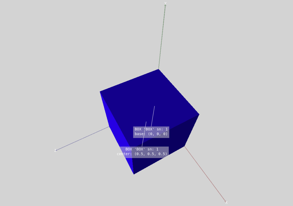
Box surface drawn on scene with center and base labels

To get full surface area of box object:

area = box.get_full_area

Or, to get volume of box object:

volume = box.get_volume

To redefine xyz0 parameter of box object:

box.xyz0 = [1, 2, 3]

To redefine only x component from xyz0:

box.xyz0[0] = 1

or:

box.x0 = 1

Similar way can be applied to other objects, using other methods.

In SPH class all methods represented both as getter and setter methods. This means, that user can define or get any property. For example:

sphere = fitsgeo.SPH([0, 0, 0], 1)  # Create sphere object from SPH class
sphere.volume = 1  # Set volume to 1

Last line will make r (radius) parameter of sphere correspond to defined volume. Same works for all other methods in SPH class.

To get value of property:

volume = sphere.volume  # Get volume of sphere

Similarly, user can redefine radius of sphere according to any other defined property.

Surface module have a global created_surfaces list, this list contains all initialized surfaces. This way, all surfaces could be easily accessed from this list and modified, or, for example, drawn all together:

for surface in created_surfaces:
        surface.draw()

This command will draw all created surfaces.

Cell module

This module provides Cell class for cells definition. Example of basic cell:

box_cell = fitsgeo.Cell(
        [-box], name="Box Cell", material=fitsgeo.MAT_WATER))

Parameters in Cell class:

• cell_def: list — list with regions and the Boolean operators, " " (blank)(AND), ":" (OR), and "#" (NOT). Parentheses "(" and ")" will be added automatically for regions

• name: str = "Cell" — name for cell object

• material: fitsgeo.Material = fitsgeo.MAT_WATER — material associated with cell (predefined MAT_WATER material by default)

• volume: float = None — volume [cm\(^3\)] of the cell

• cn: int — cell object number, automatically set after every new cell initialization, but can be changed manually after initialization (number for cells start from 100)

Cells are defined by treating regions divided by surfaces. Surface classes have overloaded "+" (__pos__) and "-" (__neg__) operators, this provides capability to define “surface sense” (see PHITS manual). These operators return surface numbers of surface objects as strings.

Example:

print(-box)  # Print string "-sn", where sn is a box.sn
print(+box)  # Print string "sn", where sn is a box.sn

region1 = [-box]  # Defines negative sense of box object (inner space)
region2 = [+box]  # Defines positive sense of box object (outer space)

The symbols " " (blank), ":", and "#" denote the intersection (AND), union (OR), and complement (NOT), operators, respectively. Let’s say that we have multiple objects (box and sphere) and we want to make cell with union of these surfaces:

import fitsgeo

# Create default scene
fitsgeo.create_scene()

box = fitsgeo.BOX()  # Box surface
sphere = fitsgeo.SPH()  # Sphere surface

# Define outer void cell
outer_cell = fitsgeo.Cell(
        [+box, ":", +sphere],
        material=fitsgeo.MAT_OUTER, name="Outer Void")
# Define union of objects
cell = fitsgeo.Cell(
        [-box, ":", -sphere], name="Union")

sphere.color = fitsgeo.YELLOW  # Just to make different colors

# Draw half transparent
box.draw(opacity=0.5)
sphere.draw(opacity=0.5)

fitsgeo.phits_export()  # Export sections to PHITS

The result of visualization in FitsGeo is on the image below.

Cell as the union of box and sphere (FitsGeo visualization)

In the FitsGeo visualization we will always see our surfaces, not cells, but after export of generated sections to PHITS and visualization using ANGEL, this will be like on the image below.

Cell as the union of box and sphere (ANGEL visualization)

Exported sections to PHITS, as well as the full input file are presented below.

Exported from FitsGeo PHITS sections

[ Material ]
    mat[1] H 2.0 O 1.0  GAS=0 $ name: 'MAT_WATER'

[ Mat Name Color ]
        mat     name    size    color
        1       {MAT\_WATER}    1.00    blue

[ Surface ]
    1   BOX  0.0 0.0 0.0  1.0 0.0 0.0  0.0 1.0 0.0  0.0 0.0 1.0 $ name: 'BOX' (box, all angles are 90deg) [x0 y0 z0] [Ax Ay Az] [Bx By Bz] [Cx Cy Cz]
    2   SPH  0.0 0.0 0.0  1.0 $ name: 'SPH' (sphere) x0 y0 z0 R

[ Cell ]
    100 -1  (1):(2) $ name: 'Outer Void'

    101 1  1.0  (-1):(-2)   $ name: 'Union'

Full PHITS input file

[ Parameters ]
        icntl = 11              # (D=0) 3:ECH 5:ALL VOID 6:SRC 7,8:GSH 11:DSH 12:DUMP

[ Source ]
        s-type = 2              # mono-energetic rectangular source
        e0 = 1                  # energy of beam [MeV]
        proj = proton   # kind of incident particle

[ Material ]
    mat[1] H 2.0 O 1.0  GAS=0 $ name: 'MAT_WATER'

[ Mat Name Color ]
        mat     name    size    color
        1       {MAT\_WATER}    1.00    blue

[ Surface ]
    1   BOX  0.0 0.0 0.0  1.0 0.0 0.0  0.0 1.0 0.0  0.0 0.0 1.0 $ name: 'BOX' (box, all angles are 90deg) [x0 y0 z0] [Ax Ay Az] [Bx By Bz] [Cx Cy Cz]
    2   SPH  0.0 0.0 0.0  1.0 $ name: 'SPH' (sphere) x0 y0 z0 R

[ Cell ]
    100 -1  (1):(2) $ name: 'Outer Void'

    101 1  1.0  (-1):(-2)   $ name: 'Union'

[ T-3Dshow ]
        title = Geometry 3D
        x0 = 0
        y0 = 0
        z0 = 0

        w-wdt = 3
        w-hgt = 3
        w-dst = 10

        w-mnw = 400                     # Number of meshes in horizontal direction.
        w-mnh = 400                     # Number of meshes in vertical direction.
        w-ang = 0

        e-the = -45
        e-phi = 24
        e-dst = 100

        l-the = 80
        l-phi = 140
        l-dst = 200*100

        file = example1_3D
        output = 3                      # (D=3) Region boundary + color
        width = 0.5                     # (D=0.5) The option defines the line thickness.
        epsout = 1

[ E n d ]

Or, we can define cells as:

import fitsgeo

fitsgeo.create_scene()

box = fitsgeo.BOX()
sphere = fitsgeo.SPH()

# Define outer void
outer_cell = fitsgeo.Cell(
        [+box + +sphere],
        material=fitsgeo.MAT_OUTER, name="Outer Void")
# Intersection of inner part of box and outer part of sphere
cell_box = fitsgeo.Cell([-box + +sphere], name="Intersection")
# Inner part of sphere
cell_sphere = fitsgeo.Cell(
        [-sphere],
        name="Inner Sphere",
        material=fitsgeo.Material.database("MAT_WATER", color="yellow"))

sphere.color = fitsgeo.YELLOW  # Just to make different colors

box.draw(opacity=0.5)
sphere.draw(opacity=0.5)

fitsgeo.phits_export()  # Export sections

Three cells are defined: first for outer void, second as the intersection of the inner part of box and outer part of sphere, third as the inner part of sphere. Note that for some other cases for particle transport one more void (or with air material) cell should be defined, which contains all objects inside. See exported to PHITS sections below.

Exported from FitsGeo PHITS sections

[ Material ]
    mat[1] H 2.0 O 1.0  GAS=0 $ name: 'MAT_WATER'
    mat[2] H 2.0 O 1.0  GAS=0 $ name: 'MAT_WATER'

[ Mat Name Color ]
        mat     name    size    color
        1       {MAT\_WATER}    1.00    blue
        2       {MAT\_WATER}    1.00    yellow

[ Surface ]
    1   BOX  0.0 0.0 0.0  1.0 0.0 0.0  0.0 1.0 0.0  0.0 0.0 1.0 $ name: 'BOX' (box, all angles are 90deg) [x0 y0 z0] [Ax Ay Az] [Bx By Bz] [Cx Cy Cz]
    2   SPH  0.0 0.0 0.0  1.0 $ name: 'SPH' (sphere) x0 y0 z0 R

[ Cell ]
    100 -1  (1 2) $ name: 'Outer Void'

    101 1  1.0  (-1 2)   $ name: 'Intersection'
    102 2  1.0  (-2)   $ name: 'Inner Sphere'

Full PHITS input file

[ Parameters ]
    icntl = 11      # (D=0) 3:ECH 5:ALL VOID 6:SRC 7,8:GSH 11:DSH 12:DUMP

[ Source ]
    s-type = 2      # mono-energetic rectangular source
    e0 = 1          # energy of beam [MeV]
    proj = proton   # kind of incident particle

[ Material ]
    mat[1] H 2.0 O 1.0  GAS=0 $ name: 'MAT_WATER'
    mat[2] H 2.0 O 1.0  GAS=0 $ name: 'MAT_WATER'

[ Mat Name Color ]
        mat     name    size    color
        1       {MAT\_WATER}    1.00    blue
        2       {MAT\_WATER}    1.00    yellow

[ Surface ]
    1   BOX  0.0 0.0 0.0  1.0 0.0 0.0  0.0 1.0 0.0  0.0 0.0 1.0 $ name: 'BOX' (box, all angles are 90deg) [x0 y0 z0] [Ax Ay Az] [Bx By Bz] [Cx Cy Cz]
    2   SPH  0.0 0.0 0.0  1.0 $ name: 'SPH' (sphere) x0 y0 z0 R

[ Cell ]
    100 -1  (1 2) $ name: 'Outer Void'

    101 1  1.0  (-1 2)   $ name: 'Intersection'
    102 2  1.0  (-2)   $ name: 'Inner Sphere'

[ T-3Dshow ]
    title = Geometry 3D
    x0 = 0
    y0 = 0
    z0 = 0

    w-wdt = 3
    w-hgt = 3
    w-dst = 10

    w-mnw = 400         # Number of meshes in horizontal direction.
    w-mnh = 400         # Number of meshes in vertical direction.
    w-ang = 0

    e-the = -45
    e-phi = 24
    e-dst = 100

    l-the = 80
    l-phi = 140
    l-dst = 200*100

    file = example_3D
    output = 3          # (D=3) Region boundary + color
    width = 0.5         # (D=0.5) The option defines the line thickness.
    epsout = 1

[ E n d ]

Another cells definition (ANGEL visualization)

Finally, just like surface and material modules, cell module provides created_cells — list with all initialized cells in it.

To get this list:

fitsgeo.created_cells

Export module

Module provides functions for export of all defined objects to MC code understandable format (only export to PHTIS for now). Example:

fitsgeo.phits_export()

This will print [ Surface ], [ Cell ] and [ Material ] sections in console (other sections may be exported in future releases). By default all sections are exported in console, but this behaviour may be configured by providing additional parameters:

• to_file: bool = False — flag to export sections to the input file (flag False by default — only export to console)

• inp_name: str = "example" — name for input file export

• export_surfaces: bool = True — flag for [ Surface ] section export

• export_materials: bool = True — flag for [ Material ] section export

• export_cells: bool = True — flag for [ Cell ] section export

Example of exporting sections to input file:

fitsgeo.phits_export(to_file=True, inp_name="example")

This will export all defined sections in one example_FitsGeo.inp file. Some sections may be excluded from export:

fitsgeo.phits_export(to_file=True, inp_name="example", export_materials=False)

This will export only [ Surface ] and [ Cell ] sections.

If some of sections not defined (some of lists with objects are empty) these sections will be skiped and warning notification in console appears. For example, if there are no cells defined notification in console will be:

No cell is defined!
created_cells list is empty!

Same for other objects.

Example 0: The Column

Illustrative example of FitsGeo usage. Very basic example of how to use FitsGeo

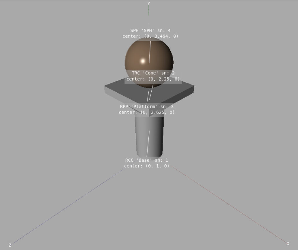
Example 0: FitsGeo visualization

Example 0: full FitsGeo code

# Example 0: The Column
# Very basic example of how to use FitsGeo
import fitsgeo as fg  # Alias to make it shorter

# Define materials from predefined databases
concrete = fg.Material.database("MAT_CONCRETE", color="gray")
bronze = fg.Material.database("MAT_BRONZE", color="pastelbrown")

fg.create_scene(ax_length=5)  # Create scene with default settings

base = fg.RCC([0, 0, 0], [0, 2, 0], name="Base", material=concrete)
cone = fg.TRC(
	base.h,
	[base.h[0]/4, base.h[1]/4, base.h[2]/4],
	r_1=base.r, r_2=base.r*2, name="Cone", material=concrete)
platform = fg.RPP(
	[-cone.r_2, cone.r_2],
	[cone.y0+cone.h[1], cone.y0+cone.h[1]+cone.get_len_h/2],
	[-cone.r_2, cone.r_2], name="Platform", material=concrete)
ball = fg.SPH(
	[platform.get_center[0],
	 platform.get_center[1]+cone.r_2/1.4+platform.get_height/2,
	 platform.get_center[2]], r=cone.r_2/1.4, material=bronze)

outer_c = fg.Cell(
	[+base + +cone + +platform + +ball], "Outer Void", fg.MAT_OUTER)
base_c = fg.Cell([-base], "Base Cell", base.material, base.get_volume)
cone_c = fg.Cell([-cone], "Cone Cell", cone.material, cone.get_volume)
platform_c = fg.Cell(
	[-platform], "Platform Cell", platform.material, platform.get_volume)
ball_c = fg.Cell([-ball], "Ball Cell", ball.material, ball.volume)

# Draw all surfaces with labels on centers
for s in fg.created_surfaces:
	s.draw(label_center=True)

# Export to PHITS
fg.phits_export(to_file=True, inp_name="example0")

In this example we will create the column as it shown on the picture above. The full FitsGeo code for this example is also shown above.

In the begining we need to import FitsGeo:

import fitsgeo as fg  # Alias to make it shorter

Here we import FitsGeo with fg alias to make it shorter. Thus, to get the FitsGeo functionality we will use fg, not fitsgeo.

First stage of geometry setup is to understand which materials we will need. In this example we only need 2 materials, which can be easily obtained through the predefined databases:

# Define materials from predefined databases
concrete = fg.Material.database("MAT_CONCRETE", color="gray")
bronze = fg.Material.database("MAT_BRONZE", color="pastelbrown")

This is concrete for column base and bronze for sphere on top. The main workflow can be as follows: find the desired materials in the Predefined Materials section, see if all properties in the database are ok, and define this material, if something is not as you expect, define this material manually, or change some property (e.g. density) in predefined material just after initialization.

After that we can create default scene as:

fg.create_scene(ax_length=5)  # Create scene with default settings

Here we make the axes longer than the ones by default. This line of code can be anywhere, except after lines with the draw method of surfaces. Also, we can just skip this line and not define the scene at all, but in this case we will not be able to change some of the scene properties, and the automatically created scene will have a black background and no axes.

Next part of code defines surfaces for geometry: cylinder, truncated cone and platform for base of column and sphere on top of that:

base = fg.RCC([0, 0, 0], [0, 2, 0], name="Base", material=concrete)
cone = fg.TRC(
	base.h,
	[base.h[0]/4, base.h[1]/4, base.h[2]/4],
	r_1=base.r, r_2=base.r*2, name="Cone", material=concrete)
platform = fg.RPP(
	[-cone.r_2, cone.r_2],
	[cone.y0+cone.h[1], cone.y0+cone.h[1]+cone.get_len_h/2],
	[-cone.r_2, cone.r_2], name="Platform", material=concrete)
ball = fg.SPH(
	[platform.get_center[0],
	 platform.get_center[1]+cone.r_2/1.4+platform.get_height/2,
	 platform.get_center[2]], r=cone.r_2/1.4, material=bronze)

Here, the advantage of FitsGeo use getting more clear: we don’t need to operate with absolute values of every surface. We can just define our “base” surface and place every other surface relatively from it (or from any other surface). Only the base has absolute values in parameters, the other surfaces are placed and sized relative to other surfaces. For example: base point of cone set as base height vector coordinates, base radius of cone set as radius of base and so on. In this case, if we change any parameter of base other surfaces changes accordingly.

After surfaces are defined, we need to define cells:

outer_c = fg.Cell(
	[+base + +cone + +platform + +ball], "Outer Void", fg.MAT_OUTER)
base_c = fg.Cell([-base], "Base Cell", base.material, base.get_volume)
cone_c = fg.Cell([-cone], "Cone Cell", cone.material, cone.get_volume)
platform_c = fg.Cell(
	[-platform], "Platform Cell", platform.material, platform.get_volume)
ball_c = fg.Cell([-ball], "Ball Cell", ball.material, ball.volume)

Here, the advantage is that we operate with names of surfaces, not with surface numbers. This make it more easy to define cells. Also, we can provide volume of cells automatically, without calculation by hand.

Finally, we can draw surfaces and export all objects to PHITS:

# Draw all surfaces with labels on centers
for s in fg.created_surfaces:
	s.draw(label_center=True)

# Export to PHITS
fg.phits_export(to_file=True, inp_name="example0")

Here, for every surface object there are labels pointing on centers. VPython visualization allows to look on geometry from every side interactively.

The following figure shows the visualization of the geometry in PHITS (via ANGEL). The full input file for PHITS is also shown below, note that the sections exported from FitsGeo are located under lines 14–37.

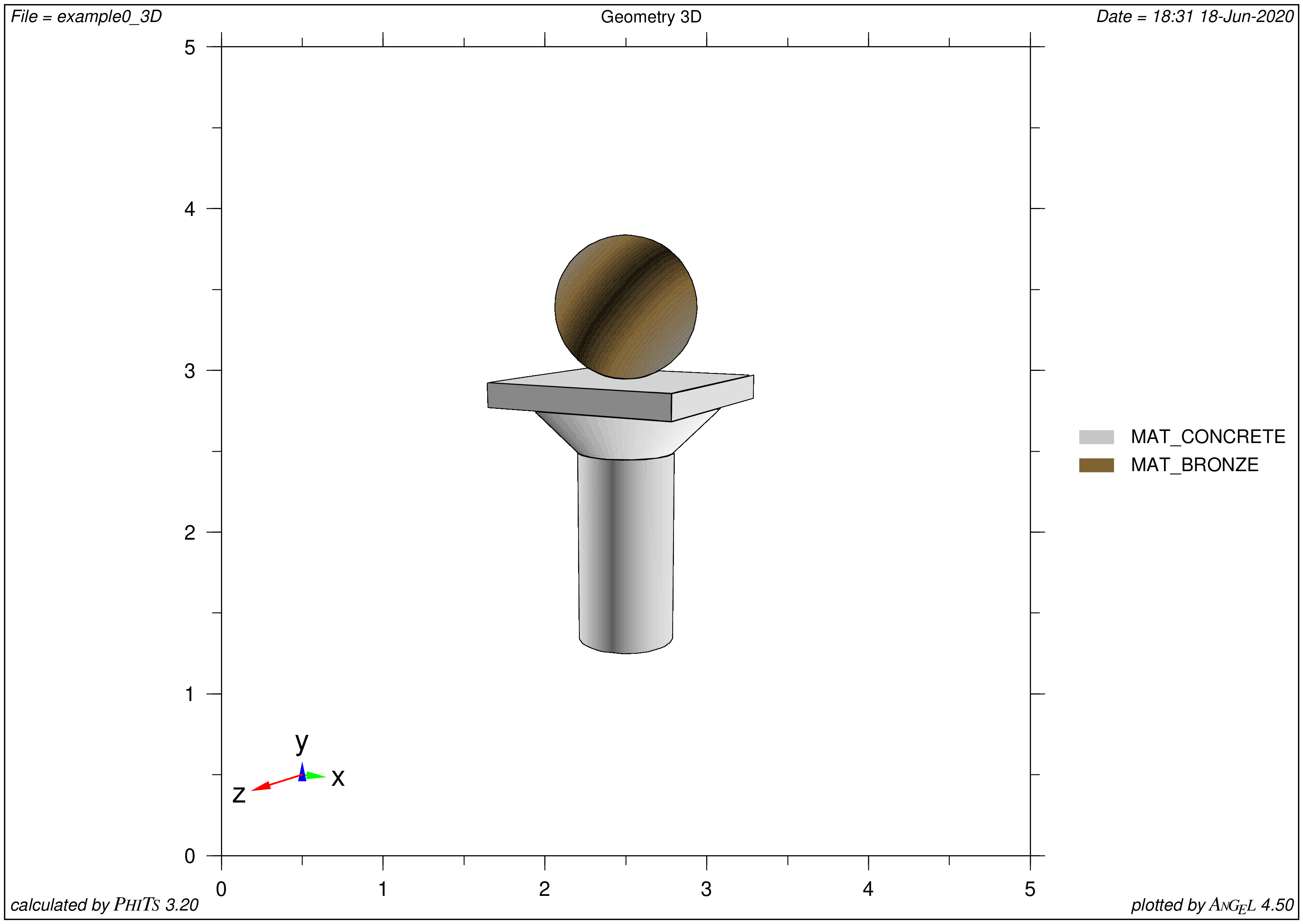
Example 0: PHITS visualization

Example 0: PHITS input

[ Title ]
	Example 0: The Column
	Illustrative example of FitsGeo usage
	Very basic example of how to use FitsGeo

[ Parameters ]
	icntl = 11		# (D=0) 3:ECH 5:ALL VOID 6:SRC 7,8:GSH 11:DSH 12:DUMP

[ Source ]
	s-type = 2		# mono-energetic rectangular source
	e0 = 1			# energy of beam [MeV]
	proj = proton	# kind of incident particle

[ Material ]
    mat[1] H 2.0 O 1.0  GAS=0 $ name: 'MAT_WATER'
    mat[2] C 23.0 O 40.0 Si 12.0 Ca 12.0 H 10.0 Mg 2.0  GAS=0 $ name: 'MAT_CONCRETE'
    mat[3] Cu 89.0 Zn 9.0 Pb 2.0  GAS=0 $ name: 'MAT_BRONZE'

[ Mat Name Color ]
        mat     name    size    color
        1       {MAT\_WATER}    1.00    blue
        2       {MAT\_CONCRETE} 1.00    gray
        3       {MAT\_BRONZE}   1.00    pastelbrown

[ Surface ]
    1   RCC  0 0 0  0 2 0  0.5 $ name: 'Base' (cylinder) [x0 y0 z0] [Hx Hy Hz] R
    2   TRC  0 2 0  0.0 0.5 0.0  0.5  1.0 $ name: 'Cone' (truncated right-angle cone) [x0 y0 z0] [Hx Hy Hz] R_b R_t
    3   RPP  -1.0 1.0  2.5 2.75  -1.0 1.0 $ name: 'Platform' (Rectangular solid) [x_min x_max] [y_min y_max] [z_min z_max]
    4   SPH  0.0 3.4642857142857144 0.0  0.7142857142857143 $ name: 'SPH' (sphere) x0 y0 z0 R

[ Cell ]
    100 -1  (1 2 3 4) $ name: 'Outer Void' 

    101 2  2.34  (-1)  VOL=1.5707963267948966 $ name: 'Base Cell' 
    102 2  2.34  (-2)  VOL=0.916297857297023 $ name: 'Cone Cell' 
    103 2  2.34  (-3)  VOL=1.0 $ name: 'Platform Cell' 
    104 3  8.82  (-4)  VOL=1.526527042560638 $ name: 'Ball Cell' 

[ T-3Dshow ]
	title = Geometry 3D
	x0 = 0
	y0 = 2
	z0 = 0

	w-wdt = 5
	w-hgt = 5
	w-dst = 4

	w-mnw = 400			# Number of meshes in horizontal direction.
	w-mnh = 400			# Number of meshes in vertical direction.
	w-ang = 0

	e-the = 30
	e-phi = 20
	e-dst = 10

	l-the = 80
	l-phi = 140
	l-dst = 200*100

	file = example0_3D
	output = 3			# (D=3) Region boundary + color
	width = 0.5			# (D=0.5) The option defines the line thickness.

	epsout = 1

[ E n d ]

Example 1: general illustrative example of FitsGeo

Illustrative example of FitsGeo usage. Covers all implemented surfaces and features

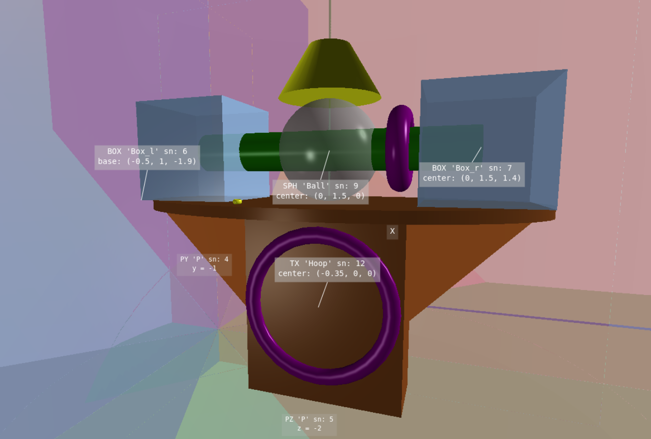
Example 1: FitsGeo visualization

In this example, we can see almost all the implemented features and aspects of work with FitsGeo. The full view on created geometry is shown in the image above. The full FitsGeo code for this example is shown below.

Example 1: full FitsGeo code

# Example 1: general illustrative example of FitsGeo
# Illustrative example of FitsGeo usage
# Covers all implemented surfaces and features
import fitsgeo as fg

fg.list_all_surfaces()  # Shows all implemented surfaces

# Create main scene with axes
ax_l = 5  # Specify axes length
scene = fg.create_scene(ax_length=ax_l)
# Change scene background
scene.background = fg.rgb_to_vector(192, 192, 192)

# Define materials from predefined databases
epoxy = fg.Material.database("MAT_EPOXY", color="pastelblue")
glass = fg.Material.database("MAT_GLASS_PB", color="gray")
al = fg.Material.database("MAT_AL", color="brown")
carbon = fg.Material.database("MAT_CARBON", color="purple")
beryllium = fg.Material.database("MAT_BE", color="green")

# Define material manually
poly = fg.Material(
	[[0, 6, 2], [0, 1, 4]], density=0.94, name="Polyethylene", color="yellow")

# Surface definitions
# Plane definition
p1 = fg.P(1, -1, -1, 4)
px1 = fg.P(0, 0, 0, 1, vert="x")
py1 = fg.P(0, 0, 0, -1, vert="y")
pz1 = fg.P(0, 0, 0, -2, vert="z")

# BOX definition
box_l = fg.BOX(
	[-1, -1, -2],
	[1, 0, 0], [0, 1, 0], [0, 0, 1], name="Box_l", material=epoxy)
box_r = fg.BOX(
	[-1, -1, -2],
	[1, 0, 0], [0, 1, 0], [0, 0, 1], name="Box_r", material=epoxy)

# RPP definition
table = fg.RPP(
	[-0.3, 0.3], [-1, 1], [-0.8, 0.8], name="Table", material=al)

# SPH definition
ball = fg.SPH([0, 1.5, 0], 0.5, name="Ball", material=glass)

# RCC definition
cyl = fg.RCC(
	[0, 0, 0], [1, 1, 1], 0.2, name="Cylinder", material=beryllium)

# TRC definition
hat = fg.TRC([0, 2, 0], [0, 0.5, 0], 0.5, 0.2, name="Hat", material=poly)

# TX definition
hoop = fg.T(
	[-3, 0, 0], 1, 0.05, 0.08, name="Hoop", rot="x", material=carbon)

# TY definition
ring = fg.T([-3, 0, 0], 0.03, 0.02, 0.01, name="Ring", material=poly)

# TZ definition
donut = fg.T(
	[0, 3, 0], 0.3, 0.1, 0.1, name="Donut", rot="z", material=carbon)

# REC definition
tabletop = fg.REC(
	[0, 0.9, 0],
	[0, 0.1, 0],
	[1, 0, 0],
	[0, 2, 0], name="Table Top", material=al)

wedge_r = fg.WED(
	[0, 0, 0], [0, -1, 0], [0, 0, 1], [1, 0, 0], name="Wedge R", material=al)
wedge_l = fg.WED(
	[0, 0, 0], [0, -1, 0], [0, 0, 1], [1, 0, 0], name="Wedge L", material=al)

# We need surface which will contain all surfaces
void = fg.RCC([0, -1.5, 0], [0, 5, 0], 3, material=fg.MAT_VOID)

# Redefine properties
box_l.xyz0 = [box_l.x0+0.5, box_l.y0+2, box_l.z0+0.1]
box_r.xyz0 = [box_r.x0+0.5, box_r.y0+2, box_r.z0+0.1]
box_r.z0 = box_r.z0+2.8

cyl.xyz0 = box_r.get_center
cyl.h = box_l.get_center - box_r.get_center

ring.xyz0 = [
	tabletop.x0 - tabletop.get_len_b/3,
	tabletop.y0 + tabletop.get_len_h + ring.b,
	tabletop.z0 - tabletop.get_len_b/3]

donut.xyz0 = [
	cyl.get_center[0], cyl.get_center[1], cyl.get_center[2] + cyl.get_len_h/4]
donut.r = cyl.r + donut.b

hoop.r = hoop.r * 0.7
hoop.x0 = -table.get_width/2 - hoop.b

table.y[1] = table.y[1] - tabletop.get_len_h

wedge_r.xyz0 = [
	table.get_center[0]-table.get_width/2,
	table.get_center[1]+table.get_height/2,
	table.get_center[2]+table.get_length/2]

wedge_r.h[0] = table.get_width

wedge_l.xyz0 = [
	table.get_center[0]+table.get_width/2,
	table.get_center[1]+table.get_height/2,
	table.get_center[2]-table.get_length/2]

wedge_l.h[0] = -table.get_width
wedge_l.b[2] = -wedge_l.b[2]

# Draw objects on scene
for p in [p1, px1, py1, pz1]:
	p.draw(size=ax_l)  # Plane will be sized according to axes

# Draw separately if some flags needed
box_l.draw(label_base=True, label_center=False, opacity=0.8)
box_r.draw(label_base=False, label_center=True, opacity=0.8)
ball.draw(label_center=True, opacity=0.6)
hoop.draw(label_center=True)

# Draw through list without additional flags
for s in [table, cyl, hat, ring, donut, tabletop, wedge_l, wedge_r, void]:
	s.draw()

# Create cells
outer_c = fg.Cell([+void], "Outer Void", fg.MAT_OUTER)

# List of surfaces inside void surface
surfaces = [
	box_l, box_r,
	table, tabletop, ball, cyl, hat, hoop, ring, donut, wedge_l, wedge_r]

# String with surfaces for cell definition
inner_surfaces = ""
for s in surfaces:
	inner_surfaces += +s

void_c = fg.Cell([-void, " ", inner_surfaces], "Void", fg.MAT_VOID)

cells = []
for s in surfaces:
	cells.append(fg.Cell([-s], name=f"{s.name} Cell", material=s.material))

# Redefine specific cells
cells[0].cell_def = [-box_l + +cyl]
cells[1].cell_def = [-box_r + +cyl]
cells[4].cell_def = [-ball + +cyl]

# Print all properties of defined surfaces
for s in fg.created_surfaces:
	s.print_properties()
	print()

# Export sections to PHITS input file
fg.phits_export(to_file=True, inp_name="example1")

First of all, we need to import FitsGeo:

import fitsgeo as fg

In line 6, we call the command to display all implemented surface classes in the console:

fg.list_all_surfaces()  # Shows all implemented surfaces

The part of the code below shows how to create and configure the scene:

# Create main scene with axes
ax_l = 5  # Specify axes length
scene = fg.create_scene(ax_length=ax_l)
# Change scene background
scene.background = fg.rgb_to_vector(192, 192, 192)

Here we use special ax_l variable for axes length. We can also change background of scene through VPython background parameter. This is a VPython color vector. In this case, background defined through rgb_to_vector function with RGB colors.

In the lines 14-23 we define materials for future geometry in two ways: from databases and manually for Polyethylene:

# Define materials from predefined databases
epoxy = fg.Material.database("MAT_EPOXY", color="pastelblue")
glass = fg.Material.database("MAT_GLASS_PB", color="gray")
al = fg.Material.database("MAT_AL", color="brown")
carbon = fg.Material.database("MAT_CARBON", color="purple")
beryllium = fg.Material.database("MAT_BE", color="green")

# Define material manually
poly = fg.Material(
	[[0, 6, 2], [0, 1, 4]], density=0.94, name="Polyethylene", color="yellow")

Starting from line 25 we define surfaces. Following part of code defines planes:

# Plane definition
p1 = fg.P(1, -1, -1, 4)
px1 = fg.P(0, 0, 0, 1, vert="x")
py1 = fg.P(0, 0, 0, -1, vert="y")
pz1 = fg.P(0, 0, 0, -2, vert="z")

Here, p1 is a general plane: a plane that is not vertical with any axis. px1, py1, pz1 — special cases of planes vertical with \(X\), \(Y\) and \(Z\) axis accordingly. If we provide vert parameter with vertical axis, only d parameter for plane equation has meaning, and other parameters in plane equation can be any. We can also define these special cases only using the general plane, not providing vert. In this example we need planes only for demonstration of feature and we don’t use them for cells definitions, but, as any other surface, plane can be used for cells definitions as well. Also, unlike to other surfaces, we don’t need to pass materials to planes, colors are set depending on vertical axis and for general plane it is a mix of colors.

In the lines 32–75 we define surfaces from every class of surface module of FitsGeo. Every surface has common with other surfaces parameters and specific ones. After that, one more void surface is defined:

# We need surface which will contain all surfaces
void = fg.RCC([0, -1.5, 0], [0, 5, 0], 3, material=fg.MAT_VOID)

We need this surface to contain all our surfaces inside. Later we will assign cell with it (this can be filled with vacuum or air material).

All defined parameters of surfaces can be changed later as shown in lines 80–115. These lines demonstrate how we can easily define new positions or sizes for our objects relative to other objects. This is the advantage of OOP way of geometry creation.

After that, we can draw all surfaces. We can use different approaches for that. Next part of code shows how to draw planes:

# Draw objects on scene
for p in [p1, px1, py1, pz1]:
	p.draw(size=ax_l)  # Plane will be sized according to axes

Since the plane has infinite dimensions, we need to pass a special size parameter to the draw method. This parameter limits plane and allows to draw this plane as square (if plane is vertical) or as parallelogram for general case.

We can draw every surface separately as it shown below:

# Draw separately if some flags needed
box_l.draw(label_base=True, label_center=False, opacity=0.8)
box_r.draw(label_base=False, label_center=True, opacity=0.8)
ball.draw(label_center=True, opacity=0.6)
hoop.draw(label_center=True)

This is useful if we need to provide some labels to specific surfaces only, or if we need to change opacity levels.

Alternatively, we can define surfaces through for cycle:

# Draw through list without additional flags
for s in [table, cyl, hat, ring, donut, tabletop, wedge_l, wedge_r, void]:
	s.draw()

This works if we don’t need to provide specific additional parameters to the draw method.

The following image shows another advantage: interactive visualization. We can see even really small parts of created geometry, like the ring on the table. And it is not so easy to obtain using only ANGEL visualization in PHITS, because we will need to change camera settings accordingly.

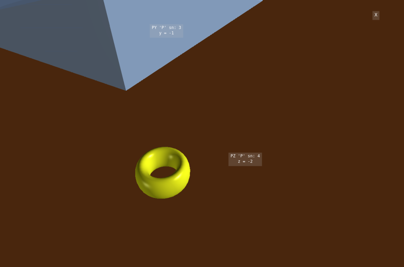
Example 1: FitsGeo visualization (ring close shot)

Starting from line 131, the part of the code with cell definitions begins. Following code defines “outer void” cell:

# Create cells
outer_c = fg.Cell([+void], "Outer Void", fg.MAT_OUTER)

In this cell transport of all particles stops.

The next part is a bit tricky:

# List of surfaces inside void surface
surfaces = [
	box_l, box_r,
	table, tabletop, ball, cyl, hat, hoop, ring, donut, wedge_l, wedge_r]

# String with surfaces for cell definition
inner_surfaces = ""
for s in surfaces:
	inner_surfaces += +s

void_c = fg.Cell([-void, " ", inner_surfaces], "Void", fg.MAT_VOID)

To define void cell we need to provide string with intersection of all inner surfaces. At first, we define surfaces list which contains all inner surfaces. After that, we create empty inner_surfaces string and loop through all surfaces in surfaces list to fill this string with intersection of all inner surfaces. And after that, in the line 144 we can finally define void cell as intersection of inner part of void surface and inner_surfaces. This way we getting cell with space in between of surfaces. It is not necessary to fill this cell with vacuum, we can fill it with air, or, whatever we need.

After that, we need to define cells for inner spaces of surfaces:

cells = []
for s in surfaces:
	cells.append(fg.Cell([-s], name=f"{s.name} Cell", material=s.material))

# Redefine specific cells
cells[0].cell_def = [-box_l + +cyl]
cells[1].cell_def = [-box_r + +cyl]
cells[4].cell_def = [-ball + +cyl]

Here, we can simply define empty cells list and append it using for loop through surfaces in list. But, this will not work for some of them: cells with box_l, box_l and ball surfaces must exclude cyl surface. Thus, we need to reconfigure cells 0, 1, 4 in cells list. Again, this is really flexible and not a problem.

The part of the code below shows how we can print all properties of surfaces in the console:

# Print all properties of defined surfaces
for s in fg.created_surfaces:
	s.print_properties()
	print()

We use the created_surfaces list for that. Every surface has a print_properties method, which prints all properties of surface in the console.

And the final part of code exports all defined sections to PHITS:

# Export sections to PHITS input file
fg.phits_export(to_file=True, inp_name="example1")

The full code of the PHITS input file, as well as the PHITS visualization, are shown below. Note that the sections exported from FitsGeo are located on the 14–68 lines.

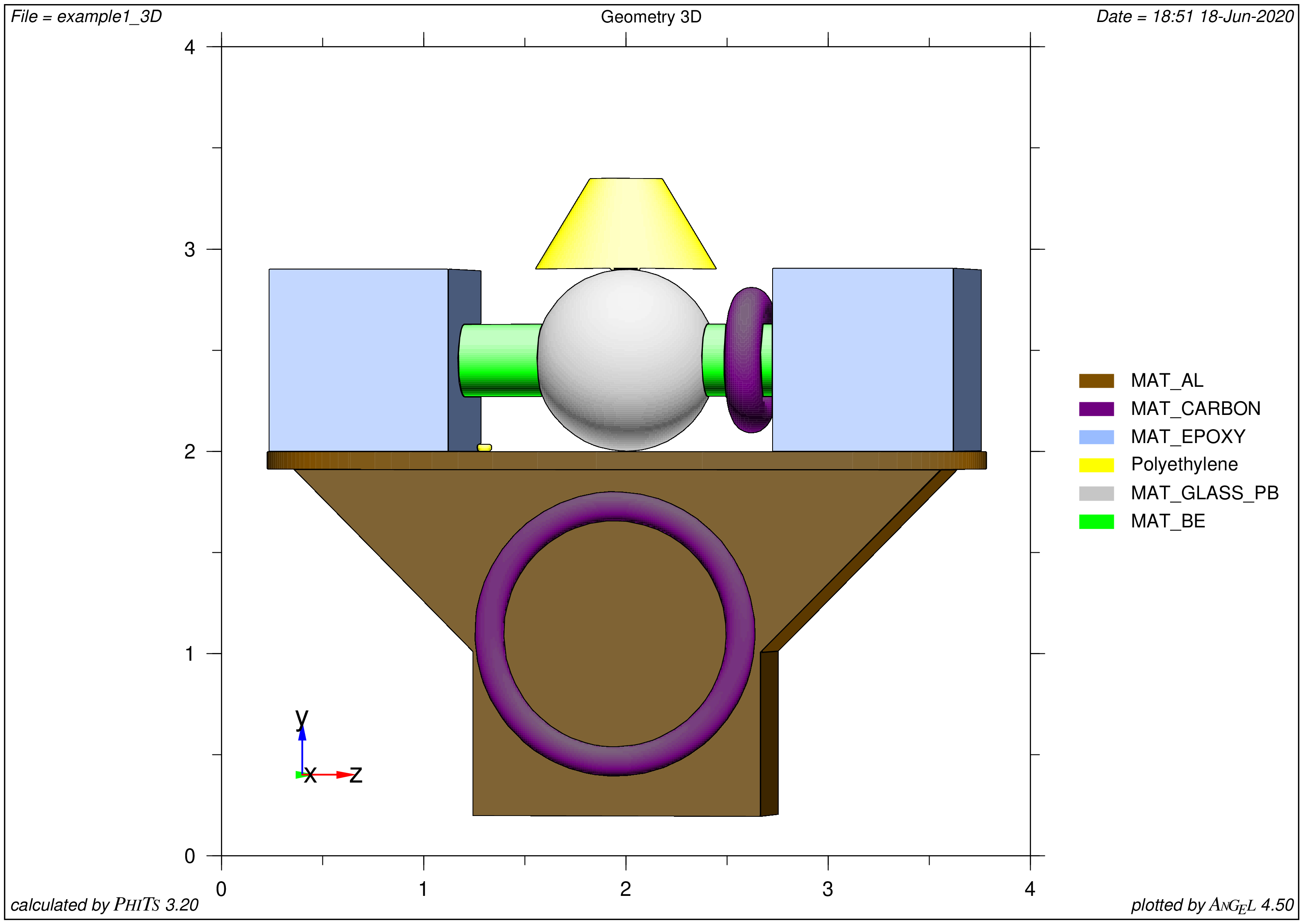
Example 1: PHITS visualization

Example 1: PHITS input

[ Title ]
	Example 1: general illustrative example of FitsGeo
	Illustrative example of FitsGeo usage
	Covers all implemented surfaces and features

[ Parameters ]
	icntl = 11		# (D=0) 3:ECH 5:ALL VOID 6:SRC 7,8:GSH 11:DSH 12:DUMP

[ Source ]
	s-type = 2		# mono-energetic rectangular source
	e0 = 1			# energy of beam [MeV]
	proj = proton	# kind of incident particle

[ Material ]
    mat[1] H 2.0 O 1.0  GAS=0 $ name: 'MAT_WATER'
    mat[2] H 19.0 C 18.0 O 3.0  GAS=0 $ name: 'MAT_EPOXY'
    mat[3] O 59.0 Si 24.0 Pb 5.0 Na 7.0 K 4.0  GAS=0 $ name: 'MAT_GLASS_PB'
    mat[4] Al 1.0  GAS=0 $ name: 'MAT_AL'
    mat[5] C 6.0  GAS=0 $ name: 'MAT_CARBON'
    mat[6] Be 1.0  GAS=0 $ name: 'MAT_BE'
    mat[7] C 2 H 4  GAS=0 $ name: 'Polyethylene'

[ Mat Name Color ]
        mat     name    size    color
        1       {MAT\_WATER}    1.00    blue
        2       {MAT\_EPOXY}    1.00    pastelblue
        3       {MAT\_GLASS\_PB}        1.00    gray
        4       {MAT\_AL}       1.00    brown
        5       {MAT\_CARBON}   1.00    purple
        6       {MAT\_BE}       1.00    green
        7       {Polyethylene}  1.00    yellow

[ Surface ]
    1   P  1 -1 -1  4 $ name: 'P' (Plane) 1x + -1y + -1z − 4 = 0
    2   PX      1 $ name: 'P' (Plane) x = 1
    3   PY      -1 $ name: 'P' (Plane) y = -1
    4   PZ      -2 $ name: 'P' (Plane) z = -2
    5   BOX  -0.5 1 -1.9  1 0 0  0 1 0  0 0 1 $ name: 'Box_l' (box, all angles are 90deg) [x0 y0 z0] [Ax Ay Az] [Bx By Bz] [Cx Cy Cz]
    6   BOX  -0.5 1 0.8999999999999999  1 0 0  0 1 0  0 0 1 $ name: 'Box_r' (box, all angles are 90deg) [x0 y0 z0] [Ax Ay Az] [Bx By Bz] [Cx Cy Cz]
    7   RPP  -0.3 0.3  -1 0.9  -0.8 0.8 $ name: 'Table' (Rectangular solid) [x_min x_max] [y_min y_max] [z_min z_max]
    8   SPH  0 1.5 0  0.5 $ name: 'Ball' (sphere) x0 y0 z0 R
    9   RCC  0.0 1.5 1.4  0.0 0.0 -2.8  0.2 $ name: 'Cylinder' (cylinder) [x0 y0 z0] [Hx Hy Hz] R
    10   TRC  0 2 0  0 0.5 0  0.5  0.2 $ name: 'Hat' (truncated right-angle cone) [x0 y0 z0] [Hx Hy Hz] R_b R_t
    11   TX  -0.35 0 0  0.7  0.05  0.08 $ name: 'Hoop' (torus, with x rotational axis) [x0 y0 z0] A(R) B C
    12   TY  -0.6666666666666666 1.02 -0.6666666666666666  0.03  0.02  0.01 $ name: 'Ring' (torus, with y rotational axis) [x0 y0 z0] A(R) B C
    13   TZ  0.0 1.5 0.7  0.30000000000000004  0.1  0.1 $ name: 'Donut' (torus, with z rotational axis) [x0 y0 z0] A(R) B C
    14   REC  0 0.9 0  0 0.1 0  1 0 0  0 2 0 $ name: 'Table Top' (elliptical cylinder) [x0 y0 z0] [Hx Hy Hz] [Ax Ay Az] [Bx By Bz]
    15   WED  -0.3 0.8999999999999999 0.8  0 -1 0  0 0 1  0.6 0 0 $ name: 'Wedge R' (wedge) [x0 y0 z0] [Ax Ay Az] [Bx By Bz] [Hx Hy Hz]
    16   WED  0.3 0.8999999999999999 -0.8  0 -1 0  0 0 -1  -0.6 0 0 $ name: 'Wedge L' (wedge) [x0 y0 z0] [Ax Ay Az] [Bx By Bz] [Hx Hy Hz]
    17   RCC  0 -1.5 0  0 5 0  3 $ name: 'RCC' (cylinder) [x0 y0 z0] [Hx Hy Hz] R

[ Cell ]
    100 -1  (17) $ name: 'Outer Void' 

    101 0  (-17) (5 6 7 14 8 9 10 11 12 13 16 15) $ name: 'Void' 

    102 2  1.18  (-5 9)   $ name: 'Box_l Cell' 
    103 2  1.18  (-6 9)   $ name: 'Box_r Cell' 
    104 4  2.6989  (-7)   $ name: 'Table Cell' 
    105 4  2.6989  (-14)   $ name: 'Table Top Cell' 
    106 3  4.8  (-8 9)   $ name: 'Ball Cell' 
    107 6  1.848  (-9)   $ name: 'Cylinder Cell' 
    108 7  0.94  (-10)   $ name: 'Hat Cell' 
    109 5  2.0  (-11)   $ name: 'Hoop Cell' 
    110 7  0.94  (-12)   $ name: 'Ring Cell' 
    111 5  2.0  (-13)   $ name: 'Donut Cell' 
    112 4  2.6989  (-16)   $ name: 'Wedge L Cell' 
    113 4  2.6989  (-15)   $ name: 'Wedge R Cell' 

[ T-3Dshow ]
	title = Geometry 3D
	x0 = 0
	y0 = 1
	z0 = 0

	w-wdt = 4
	w-hgt = 4
	w-dst = 10

	w-mnw = 400			# Number of meshes in horizontal direction.
	w-mnh = 400			# Number of meshes in vertical direction.
	w-ang = 0

	e-the = -80
	e-phi = 0
	e-dst = 100

	l-the = 80
	l-phi = 140
	l-dst = 200*100

	file = example1_3D
	output = 3			# (D=3) Region boundary + color
	width = 0.5			# (D=0.5) The option defines the line thickness.
	epsout = 1

[ E n d ]

Example 2(a): Spheres with Hats

Illustrative example of FitsGeo usage. Shows how to easily create multiple (repeating) objects

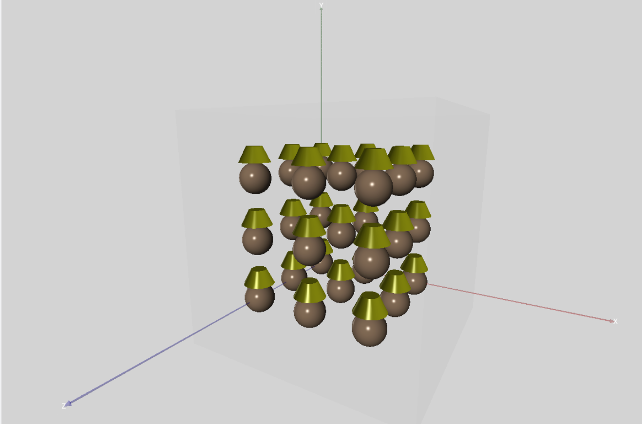
Example 2(a): FitsGeo visualization

In this example, the creation of geometry with multiple (repeating) surfaces using FitsGeo is shown. The visualization in FitsGeo of created geometry is shown in the image above. The full FitsGeo code for this example is shown below.

Example 2(a): full FitsGeo code

# Example 2(a): Spheres with Hats
# Illustrative example of FitsGeo usage
# Shows how to easily create multiple (repeating) objects
import fitsgeo as fg

# Create main scene, with axes
fg.create_scene(ax_length=10)

# Define materials
gold = fg.Material.database("MAT_AU", color="yellow")
bronze = fg.Material.database("MAT_BRONZE", color="pastelbrown")

spheres, hats = [], []  # Lists for surfaces

n = 3  # Number of objects along each axis

cells = []  # List for cells
i = 0
for z in range(n):
	for y in range(n):
		for x in range(n):
			s = fg.SPH(
					[x + (1 * x), y + (1 * y), z + (1 * z)],
					0.5, material=bronze)
			spheres.append(s)
			cells.append(fg.Cell([-s], f"Cell SPH {i}", s.material, s.volume))

			# Parameters for hat
			hat_h = spheres[i].r
			hat_r = spheres[i].diameter / 2
			hat_x0 = spheres[i].x0
			hat_y0 = spheres[i].y0 + hat_h
			hat_z0 = spheres[i].z0

			s = fg.TRC(
					[hat_x0, hat_y0, hat_z0],
					[0, hat_h, 0], hat_r, hat_r/2, material=gold)
			hats.append(s)
			cells.append(fg.Cell([-s], f"Cell TRC {i}", s.material, s.get_volume))
			i += 1

# Void definition
inner_surfaces = ""
for s in fg.created_surfaces:
	inner_surfaces += +s

void_s = fg.RPP(
	[-1, 6], [-1, 6], [-1, 6], "Void Surface", material=fg.MAT_VOID)

outer_c = fg.Cell(
	[+void_s], "Outer Cell", fg.MAT_OUTER)

void_c = fg.Cell(
	[-void_s, " ", inner_surfaces], "Void Cell", void_s.material)

# Draw surfaces
for i in range(n**3):
	spheres[i].draw()
	hats[i].draw(truncated=True)
void_s.draw()

fg.phits_export(to_file=True, inp_name="example2a")

Like always, the first thing to do is to import FitsGeo:

import fitsgeo as fg

Create scene with 10 cm of axes length:

# Create main scene, with axes
fg.create_scene(ax_length=10)

Define 2 materials from predefined databases with "yellow" and "pastelbrown" colors for future spheres and their “hats”:

# Define materials
gold = fg.Material.database("MAT_AU", color="yellow")
bronze = fg.Material.database("MAT_BRONZE", color="pastelbrown")

After these preparation steps, let’s say we need some structure with repeating parts. In this example, these are spheres and “hats” on top of these spheres. With the help of Python and object-oriented way of geometry development, this will be easy. First, let’s create empty lists for future surfaces and cells and set how many objects we need along each axis:

spheres, hats = [], []  # Lists for surfaces

n = 3  # Number of objects along each axis

cells = []  # List for cells

The next part of code have 3 for loops:

i = 0
for z in range(n):
	for y in range(n):
		for x in range(n):
			s = fg.SPH(
					[x + (1 * x), y + (1 * y), z + (1 * z)],
					0.5, material=bronze)
			spheres.append(s)
			cells.append(fg.Cell([-s], f"Cell SPH {i}", s.material, s.volume))

			# Parameters for hat
			hat_h = spheres[i].r
			hat_r = spheres[i].diameter / 2
			hat_x0 = spheres[i].x0
			hat_y0 = spheres[i].y0 + hat_h
			hat_z0 = spheres[i].z0

			s = fg.TRC(
					[hat_x0, hat_y0, hat_z0],
					[0, hat_h, 0], hat_r, hat_r/2, material=gold)
			hats.append(s)
			cells.append(fg.Cell([-s], f"Cell TRC {i}", s.material, s.get_volume))
			i += 1

On each iteration we define one more sphere with hat: surface and cell objects for each of them. Parameters for every new hat are set according to sphere parameters.

The rest part of the code (lines 42–62) defines last cell objects for void and “outer void”, draws all surfaces and exports sections to PHITS input, just like it was done in the examples discussed previously. Similarly, we can easily create more repeating objects depending on our needs.

Full PHITS input file and visualization of geometry via ANGEL are shown below. The highlighted part of the code — exported sections from FitsGeo.

Example 2(a): PHITS input

[ Title ]
	Example 2(a): Spheres with Hats
	Illustrative example of FitsGeo usage
	Shows how to create multiple (repeating) objects

[ Parameters ]
	icntl = 11		# (D=0) 3:ECH 5:ALL VOID 6:SRC 7,8:GSH 11:DSH 12:DUMP

[ Source ]
	s-type = 2		# mono-energetic rectangular source
	e0 = 1			# energy of beam [MeV]
	proj = proton	# kind of incident particle

[ Material ]
    mat[1] H 2.0 O 1.0  GAS=0 $ name: 'MAT_WATER'
    mat[2] Au 1.0  GAS=0 $ name: 'MAT_AU'
    mat[3] Cu 89.0 Zn 9.0 Pb 2.0  GAS=0 $ name: 'MAT_BRONZE'

[ Mat Name Color ]
    mat name    size    color
    1   {MAT\_WATER}    1.00    blue
    2   {MAT\_AU}   1.00    yellow
    3   {MAT\_BRONZE}   1.00    pastelbrown

[ Surface ]
    1   SPH  0 0 0  0.5 $ name: 'SPH' (sphere) x0 y0 z0 R
    2   TRC  0 0.5 0  0 0.5 0  0.5  0.25 $ name: 'RCC' (truncated right-angle cone) [x0 y0 z0] [Hx Hy Hz] R_b R_t
    3   SPH  2 0 0  0.5 $ name: 'SPH' (sphere) x0 y0 z0 R
    4   TRC  2 0.5 0  0 0.5 0  0.5  0.25 $ name: 'RCC' (truncated right-angle cone) [x0 y0 z0] [Hx Hy Hz] R_b R_t
    5   SPH  4 0 0  0.5 $ name: 'SPH' (sphere) x0 y0 z0 R
    6   TRC  4 0.5 0  0 0.5 0  0.5  0.25 $ name: 'RCC' (truncated right-angle cone) [x0 y0 z0] [Hx Hy Hz] R_b R_t
    7   SPH  0 2 0  0.5 $ name: 'SPH' (sphere) x0 y0 z0 R
    8   TRC  0 2.5 0  0 0.5 0  0.5  0.25 $ name: 'RCC' (truncated right-angle cone) [x0 y0 z0] [Hx Hy Hz] R_b R_t
    9   SPH  2 2 0  0.5 $ name: 'SPH' (sphere) x0 y0 z0 R
    10   TRC  2 2.5 0  0 0.5 0  0.5  0.25 $ name: 'RCC' (truncated right-angle cone) [x0 y0 z0] [Hx Hy Hz] R_b R_t
    11   SPH  4 2 0  0.5 $ name: 'SPH' (sphere) x0 y0 z0 R
    12   TRC  4 2.5 0  0 0.5 0  0.5  0.25 $ name: 'RCC' (truncated right-angle cone) [x0 y0 z0] [Hx Hy Hz] R_b R_t
    13   SPH  0 4 0  0.5 $ name: 'SPH' (sphere) x0 y0 z0 R
    14   TRC  0 4.5 0  0 0.5 0  0.5  0.25 $ name: 'RCC' (truncated right-angle cone) [x0 y0 z0] [Hx Hy Hz] R_b R_t
    15   SPH  2 4 0  0.5 $ name: 'SPH' (sphere) x0 y0 z0 R
    16   TRC  2 4.5 0  0 0.5 0  0.5  0.25 $ name: 'RCC' (truncated right-angle cone) [x0 y0 z0] [Hx Hy Hz] R_b R_t
    17   SPH  4 4 0  0.5 $ name: 'SPH' (sphere) x0 y0 z0 R
    18   TRC  4 4.5 0  0 0.5 0  0.5  0.25 $ name: 'RCC' (truncated right-angle cone) [x0 y0 z0] [Hx Hy Hz] R_b R_t
    19   SPH  0 0 2  0.5 $ name: 'SPH' (sphere) x0 y0 z0 R
    20   TRC  0 0.5 2  0 0.5 0  0.5  0.25 $ name: 'RCC' (truncated right-angle cone) [x0 y0 z0] [Hx Hy Hz] R_b R_t
    21   SPH  2 0 2  0.5 $ name: 'SPH' (sphere) x0 y0 z0 R
    22   TRC  2 0.5 2  0 0.5 0  0.5  0.25 $ name: 'RCC' (truncated right-angle cone) [x0 y0 z0] [Hx Hy Hz] R_b R_t
    23   SPH  4 0 2  0.5 $ name: 'SPH' (sphere) x0 y0 z0 R
    24   TRC  4 0.5 2  0 0.5 0  0.5  0.25 $ name: 'RCC' (truncated right-angle cone) [x0 y0 z0] [Hx Hy Hz] R_b R_t
    25   SPH  0 2 2  0.5 $ name: 'SPH' (sphere) x0 y0 z0 R
    26   TRC  0 2.5 2  0 0.5 0  0.5  0.25 $ name: 'RCC' (truncated right-angle cone) [x0 y0 z0] [Hx Hy Hz] R_b R_t
    27   SPH  2 2 2  0.5 $ name: 'SPH' (sphere) x0 y0 z0 R
    28   TRC  2 2.5 2  0 0.5 0  0.5  0.25 $ name: 'RCC' (truncated right-angle cone) [x0 y0 z0] [Hx Hy Hz] R_b R_t
    29   SPH  4 2 2  0.5 $ name: 'SPH' (sphere) x0 y0 z0 R
    30   TRC  4 2.5 2  0 0.5 0  0.5  0.25 $ name: 'RCC' (truncated right-angle cone) [x0 y0 z0] [Hx Hy Hz] R_b R_t
    31   SPH  0 4 2  0.5 $ name: 'SPH' (sphere) x0 y0 z0 R
    32   TRC  0 4.5 2  0 0.5 0  0.5  0.25 $ name: 'RCC' (truncated right-angle cone) [x0 y0 z0] [Hx Hy Hz] R_b R_t
    33   SPH  2 4 2  0.5 $ name: 'SPH' (sphere) x0 y0 z0 R
    34   TRC  2 4.5 2  0 0.5 0  0.5  0.25 $ name: 'RCC' (truncated right-angle cone) [x0 y0 z0] [Hx Hy Hz] R_b R_t
    35   SPH  4 4 2  0.5 $ name: 'SPH' (sphere) x0 y0 z0 R
    36   TRC  4 4.5 2  0 0.5 0  0.5  0.25 $ name: 'RCC' (truncated right-angle cone) [x0 y0 z0] [Hx Hy Hz] R_b R_t
    37   SPH  0 0 4  0.5 $ name: 'SPH' (sphere) x0 y0 z0 R
    38   TRC  0 0.5 4  0 0.5 0  0.5  0.25 $ name: 'RCC' (truncated right-angle cone) [x0 y0 z0] [Hx Hy Hz] R_b R_t
    39   SPH  2 0 4  0.5 $ name: 'SPH' (sphere) x0 y0 z0 R
    40   TRC  2 0.5 4  0 0.5 0  0.5  0.25 $ name: 'RCC' (truncated right-angle cone) [x0 y0 z0] [Hx Hy Hz] R_b R_t
    41   SPH  4 0 4  0.5 $ name: 'SPH' (sphere) x0 y0 z0 R
    42   TRC  4 0.5 4  0 0.5 0  0.5  0.25 $ name: 'RCC' (truncated right-angle cone) [x0 y0 z0] [Hx Hy Hz] R_b R_t
    43   SPH  0 2 4  0.5 $ name: 'SPH' (sphere) x0 y0 z0 R
    44   TRC  0 2.5 4  0 0.5 0  0.5  0.25 $ name: 'RCC' (truncated right-angle cone) [x0 y0 z0] [Hx Hy Hz] R_b R_t
    45   SPH  2 2 4  0.5 $ name: 'SPH' (sphere) x0 y0 z0 R
    46   TRC  2 2.5 4  0 0.5 0  0.5  0.25 $ name: 'RCC' (truncated right-angle cone) [x0 y0 z0] [Hx Hy Hz] R_b R_t
    47   SPH  4 2 4  0.5 $ name: 'SPH' (sphere) x0 y0 z0 R
    48   TRC  4 2.5 4  0 0.5 0  0.5  0.25 $ name: 'RCC' (truncated right-angle cone) [x0 y0 z0] [Hx Hy Hz] R_b R_t
    49   SPH  0 4 4  0.5 $ name: 'SPH' (sphere) x0 y0 z0 R
    50   TRC  0 4.5 4  0 0.5 0  0.5  0.25 $ name: 'RCC' (truncated right-angle cone) [x0 y0 z0] [Hx Hy Hz] R_b R_t
    51   SPH  2 4 4  0.5 $ name: 'SPH' (sphere) x0 y0 z0 R
    52   TRC  2 4.5 4  0 0.5 0  0.5  0.25 $ name: 'RCC' (truncated right-angle cone) [x0 y0 z0] [Hx Hy Hz] R_b R_t
    53   SPH  4 4 4  0.5 $ name: 'SPH' (sphere) x0 y0 z0 R
    54   TRC  4 4.5 4  0 0.5 0  0.5  0.25 $ name: 'RCC' (truncated right-angle cone) [x0 y0 z0] [Hx Hy Hz] R_b R_t
    55   RPP  -1 6  -1 6  -1 6 $ name: 'Void Surface' (Rectangular solid) [x_min x_max] [y_min y_max] [z_min z_max]

[ Cell ]
    100 3  8.82  (-1)  VOL=0.5235987755982988 $ name: 'Cell SPH 0' 
    101 2  19.32  (-2)  VOL=0.22907446432425574 $ name: 'Cell TRC 0' 
    102 3  8.82  (-3)  VOL=0.5235987755982988 $ name: 'Cell SPH 1' 
    103 2  19.32  (-4)  VOL=0.22907446432425574 $ name: 'Cell TRC 1' 
    104 3  8.82  (-5)  VOL=0.5235987755982988 $ name: 'Cell SPH 2' 
    105 2  19.32  (-6)  VOL=0.22907446432425574 $ name: 'Cell TRC 2' 
    106 3  8.82  (-7)  VOL=0.5235987755982988 $ name: 'Cell SPH 3' 
    107 2  19.32  (-8)  VOL=0.22907446432425574 $ name: 'Cell TRC 3' 
    108 3  8.82  (-9)  VOL=0.5235987755982988 $ name: 'Cell SPH 4' 
    109 2  19.32  (-10)  VOL=0.22907446432425574 $ name: 'Cell TRC 4' 
    110 3  8.82  (-11)  VOL=0.5235987755982988 $ name: 'Cell SPH 5' 
    111 2  19.32  (-12)  VOL=0.22907446432425574 $ name: 'Cell TRC 5' 
    112 3  8.82  (-13)  VOL=0.5235987755982988 $ name: 'Cell SPH 6' 
    113 2  19.32  (-14)  VOL=0.22907446432425574 $ name: 'Cell TRC 6' 
    114 3  8.82  (-15)  VOL=0.5235987755982988 $ name: 'Cell SPH 7' 
    115 2  19.32  (-16)  VOL=0.22907446432425574 $ name: 'Cell TRC 7' 
    116 3  8.82  (-17)  VOL=0.5235987755982988 $ name: 'Cell SPH 8' 
    117 2  19.32  (-18)  VOL=0.22907446432425574 $ name: 'Cell TRC 8' 
    118 3  8.82  (-19)  VOL=0.5235987755982988 $ name: 'Cell SPH 9' 
    119 2  19.32  (-20)  VOL=0.22907446432425574 $ name: 'Cell TRC 9' 
    120 3  8.82  (-21)  VOL=0.5235987755982988 $ name: 'Cell SPH 10' 
    121 2  19.32  (-22)  VOL=0.22907446432425574 $ name: 'Cell TRC 10' 
    122 3  8.82  (-23)  VOL=0.5235987755982988 $ name: 'Cell SPH 11' 
    123 2  19.32  (-24)  VOL=0.22907446432425574 $ name: 'Cell TRC 11' 
    124 3  8.82  (-25)  VOL=0.5235987755982988 $ name: 'Cell SPH 12' 
    125 2  19.32  (-26)  VOL=0.22907446432425574 $ name: 'Cell TRC 12' 
    126 3  8.82  (-27)  VOL=0.5235987755982988 $ name: 'Cell SPH 13' 
    127 2  19.32  (-28)  VOL=0.22907446432425574 $ name: 'Cell TRC 13' 
    128 3  8.82  (-29)  VOL=0.5235987755982988 $ name: 'Cell SPH 14' 
    129 2  19.32  (-30)  VOL=0.22907446432425574 $ name: 'Cell TRC 14' 
    130 3  8.82  (-31)  VOL=0.5235987755982988 $ name: 'Cell SPH 15' 
    131 2  19.32  (-32)  VOL=0.22907446432425574 $ name: 'Cell TRC 15' 
    132 3  8.82  (-33)  VOL=0.5235987755982988 $ name: 'Cell SPH 16' 
    133 2  19.32  (-34)  VOL=0.22907446432425574 $ name: 'Cell TRC 16' 
    134 3  8.82  (-35)  VOL=0.5235987755982988 $ name: 'Cell SPH 17' 
    135 2  19.32  (-36)  VOL=0.22907446432425574 $ name: 'Cell TRC 17' 
    136 3  8.82  (-37)  VOL=0.5235987755982988 $ name: 'Cell SPH 18' 
    137 2  19.32  (-38)  VOL=0.22907446432425574 $ name: 'Cell TRC 18' 
    138 3  8.82  (-39)  VOL=0.5235987755982988 $ name: 'Cell SPH 19' 
    139 2  19.32  (-40)  VOL=0.22907446432425574 $ name: 'Cell TRC 19' 
    140 3  8.82  (-41)  VOL=0.5235987755982988 $ name: 'Cell SPH 20' 
    141 2  19.32  (-42)  VOL=0.22907446432425574 $ name: 'Cell TRC 20' 
    142 3  8.82  (-43)  VOL=0.5235987755982988 $ name: 'Cell SPH 21' 
    143 2  19.32  (-44)  VOL=0.22907446432425574 $ name: 'Cell TRC 21' 
    144 3  8.82  (-45)  VOL=0.5235987755982988 $ name: 'Cell SPH 22' 
    145 2  19.32  (-46)  VOL=0.22907446432425574 $ name: 'Cell TRC 22' 
    146 3  8.82  (-47)  VOL=0.5235987755982988 $ name: 'Cell SPH 23' 
    147 2  19.32  (-48)  VOL=0.22907446432425574 $ name: 'Cell TRC 23' 
    148 3  8.82  (-49)  VOL=0.5235987755982988 $ name: 'Cell SPH 24' 
    149 2  19.32  (-50)  VOL=0.22907446432425574 $ name: 'Cell TRC 24' 
    150 3  8.82  (-51)  VOL=0.5235987755982988 $ name: 'Cell SPH 25' 
    151 2  19.32  (-52)  VOL=0.22907446432425574 $ name: 'Cell TRC 25' 
    152 3  8.82  (-53)  VOL=0.5235987755982988 $ name: 'Cell SPH 26' 
    153 2  19.32  (-54)  VOL=0.22907446432425574 $ name: 'Cell TRC 26' 
    154 -1  (55) $ name: 'Outer Cell' 

    155 0  (-55) (1 2 3 4 5 6 7 8 9 10 11 12 13 14 15 16 17 18 19 20 21 22 23 24 25 26 27 28 29 30 31 32 33 34 35 36 37 38 39 40 41 42 43 44 45 46 47 48 49 50 51 52 53 54) $ name: 'Void Cell' 

[ T-3Dshow ]
	title = Geometry 3D
	x0 = 0
	y0 = 0
	z0 = 0

	w-wdt = 10
	w-hgt = 10
	w-dst = 10

	w-mnw = 400			# Number of meshes in horizontal direction.
	w-mnh = 400			# Number of meshes in vertical direction.
	w-ang = 0

	e-the = 45
	e-phi = 45
	e-dst = 20

	l-the = 80
	l-phi = 140
	l-dst = 200*100

	file = example2a_3D
	output = 3			# (D=3) Region boundary + color
	width = 0.5			# (D=0.5) The option defines the line thickness.

	epsout = 1

[ E n d ]

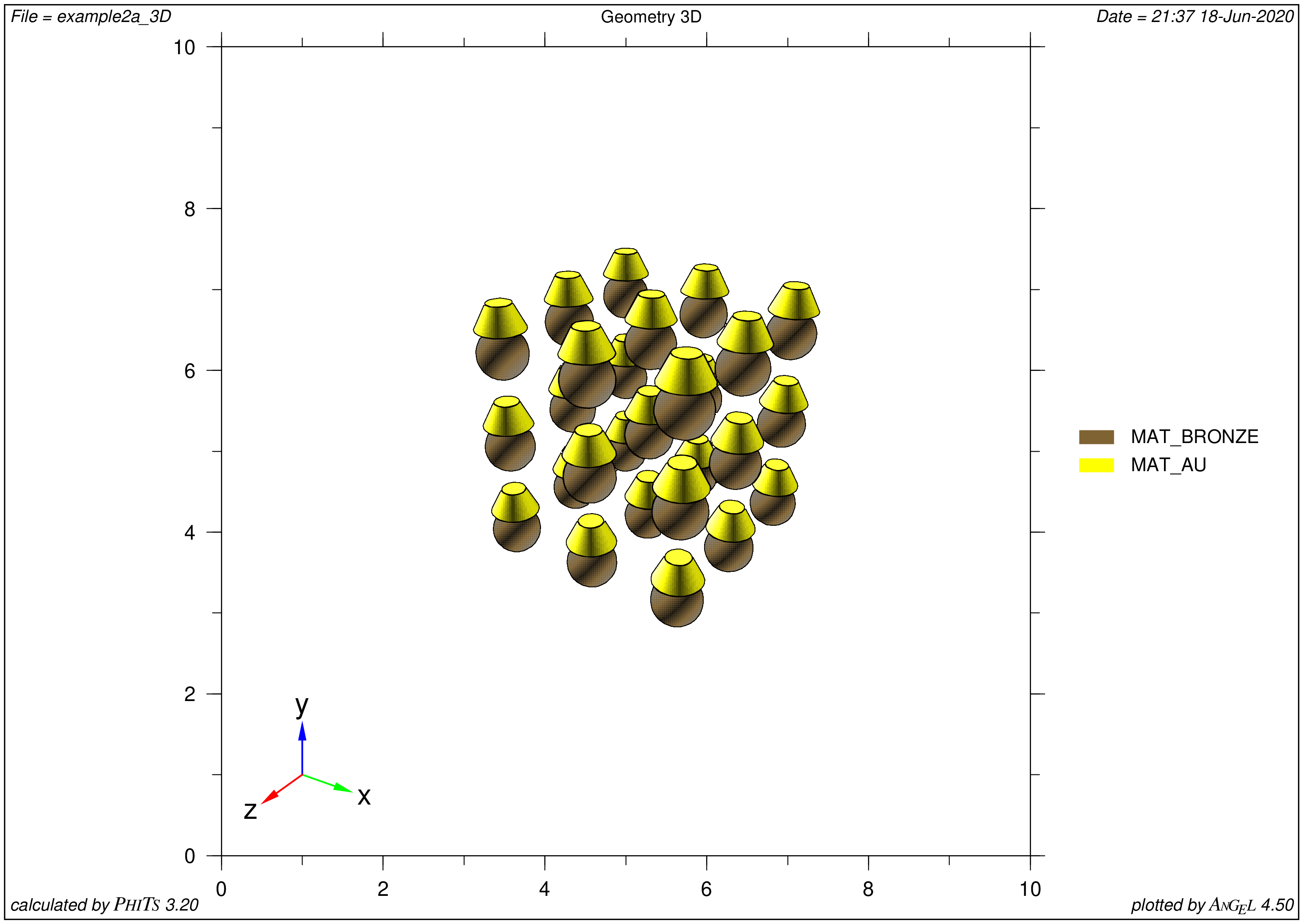
Example 2(a): PHITS visualization

Example 2(b): Snake!

Illustrative example of FitsGeo usage. Shows how to create multiple (repeating) objects according to some math laws

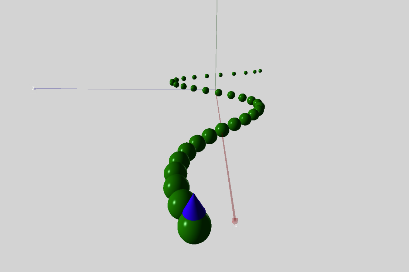
Example 2(b): Snake! FitsGeo visualization

This example shows how we can define multiple surface objects according to some math laws. The final result of visualization via FitsGeo is in the picture above. The full code of the example is shown below.

Example 2(b): Snake!

# Example 2b: Snake!
# Illustrative example of FitsGeo usage
# Shows how to easily create multiple (repeating) objects with some math laws
import fitsgeo as fg
from numpy import sin, exp, linspace  # To use math functions

# Create laws for positions of snakes parts
x = linspace(0, 5, 50)  # Create 50 evenly spaced x values from 0 to 5
# Law for z coordinate
z_p = [5 * sin(3 * x_i) * 0.3 * exp(-0.4 * x_i) for x_i in x]
r = [0.02 * exp(0.2 * x_i) for x_i in x]  # Law for radius of spheres

# Define materials for snake and hat
snake_mat = fg.Material.database("MAT_SKIN_ICRP", color="green")
hat_mat = fg.Material.database("MAT_POLYETHYLENE", color="blue")

snake = []  # List with all parts of snake
for i in range(16, len(x)):  # Take x values starting from i=16
	snake.append(
		fg.SPH(xyz0=[x[i] - 3, 0, z_p[i]], r=r[i], material=snake_mat))

last_part = snake[len(snake)-1]
hat = fg.TRC(
	xyz0=[
		last_part.x0,
		last_part.y0 + last_part.r,
		last_part.z0],
	h=[0, last_part.diameter/1.5, 0],
	r_1=last_part.r/1.5,
	r_2=1e-9, material=hat_mat)

void = fg.RCC(
	xyz0=[
		snake[0].x0-0.1,
		snake[0].y0,
		snake[0].z0], h=[4, 0, 0], r=3, material=fg.MAT_VOID)

# Define cells
outer_void = fg.Cell([+void], material=fg.MAT_OUTER)
cells = []
for i in range(len(snake)):
	cells.append(
		fg.Cell([-snake[i]], name=f"Snake Part {i}", material=snake_mat))
# Add a nice hat on head =)
hat_cell = fg.Cell([-hat], name="Hat!", material=hat_mat)

text = ""
for s in snake:
	text += +s

void_cell = fg.Cell(
	[-void, " ", text + +hat], name="Vacuum", material=fg.MAT_VOID)

fg.create_scene(ax_length=5)  # Create scene before draw

# Draw snake
for s in snake:
	s.draw()
hat.draw(truncated=False)  # Difficulties with truncated cone =(
void.draw()

fg.phits_export(to_file=True, inp_name="snake")  # Export sections

Just like in the previous examples, we need to import FitsGeo first:

import fitsgeo as fg

After that, we need to import some additional functions from numpy package:

from numpy import sin, exp, linspace  # To use math functions

This gives us some mathematical functions with which we can define mathematical expressions later.

So, let’s say we need to define geometry of snake (why not?). This snake will have some number of body segments — spheres. Also, to make this example a bit more harder (and funnier), let’s say that we want to put a small hat on the snake’s head.

Segments of the snake’s body will be placed and sized according to the defined mathematical laws. Equation for positions of sphere segments on the \(xz\)-plane:

\(z(x) = 5\cdot\sin(3x)\cdot0.3\exp(-0.4x)\)

And on the \(y\) coordinate it is 0 everywhere (but we can define some law for this coordinate as well). The graph for this equation is in the figure below.

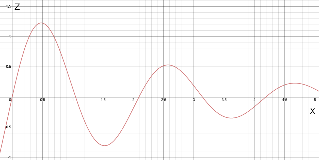
Math law for positions of snake’s segments (spheres)

The law for radius of spheres:

\(r(x) = 0.02\exp(0.2x)\)

This law will give us slow exponential (almost linear) increase in the radius of spheres depending on the \(x\) coordinate. The graph for this law is on the figure below.

Math law for radiuses of snake’s segments (spheres)

Part of the Python code for math expressions:

# Create laws for positions of snakes parts
x = linspace(0, 5, 50)  # Create 50 evenly spaced x values from 0 to 5
# Law for z coordinate
z_p = [5 * sin(3 * x_i) * 0.3 * exp(-0.4 * x_i) for x_i in x]
r = [0.02 * exp(0.2 * x_i) for x_i in x]  # Law for radius of spheres

Here, we create 50 evenly spaced \(x\) values from 0 to 5. And define laws according to the equations above.

In the lines 13–15 we define materials for snake:

# Define materials for snake and hat
snake_mat = fg.Material.database("MAT_SKIN_ICRP", color="green")
hat_mat = fg.Material.database("MAT_POLYETHYLENE", color="blue")

This time let it be ICRP skin for body segments and polyethylene for hat from predefined databases.

Next part of the code will generate sphere segments according to laws for positions and radiuses:

snake = []  # List with all parts of snake
for i in range(16, len(x)):  # Take x values starting from i=16
	snake.append(
		fg.SPH(xyz0=[x[i] - 3, 0, z_p[i]], r=r[i], material=snake_mat))

Each new iteration appends new part of body with specific position and radius to the snake list. Pay attention, that here we use \(x\) values from i=16 and make a shift by 3 by the \(x\) coordinate in case to place our snake almost in the center of coordinates.

In lines 22–30 we create our “hardest” part with placing the hat on top of the snake’s head. This task isn’t actually hard with FitsGeo:

last_part = snake[len(snake)-1]
hat = fg.TRC(
	xyz0=[
		last_part.x0,
		last_part.y0 + last_part.r,
		last_part.z0],
	h=[0, last_part.diameter/1.5, 0],
	r_1=last_part.r/1.5,
	r_2=1e-9, material=hat_mat)

All we need is to take the last part of snake list — the head of snake (line 22). After that we can create the cone (hat) with parameters relative to that snake’s head.

Last part of the code is about the same as in the another examples. Here we define void surface object, outer_void cell object, cells for every part of snake and for the hat. Define scene with 5 axes length, draw all surfaces and export everything to the file.

In the line 59 we use special parameter for hat visualization. In current release visualization of truncated cone might lead to some unstability: sometimes these cones are drawn not as expected with different sizes. To avoid this, we can set truncated parameter to False state, in that case even if cone is truncated, visualization will be performed as for the not truncated case:

hat.draw(truncated=False)  # Difficulties with truncated cone =(

Full PHITS input file and visualization of geometry via ANGEL are shown below. The highlighted part of the code — exported sections from FitsGeo.

Example 2(b): Snake! PHITS input

[ Title ]
    Example2b: Snake!
    Illustrative example of FitsGeo usage
    Shows how to create multiple (repeating) objects with some math laws

[ Parameters ]
	icntl = 11		# (D=0) 3:ECH 5:ALL VOID 6:SRC 7,8:GSH 11:DSH 12:DUMP
    #icntl = 0      # (D=0) 3:ECH 5:ALL VOID 6:SRC 7,8:GSH 11:DSH 12:DUMP
    itall = 1
    istdev = -1     # (D=0) Control parameter for statistical uncertainty calculation type and restart mode.
    negs = 1

    maxcas = 1000    # (D=10) number of particles per one batch
    maxbch = 100000     # (D=10) number of batches

[ Source ]
	s-type = 9		
	proj = proton
    x0 = 2
    y0 = 0
    z0 = 0.132
	e0 = 100.0	         
    r0 = 0.0      
    dir = all            

[ Material ]
    mat[1] H 2.0 O 1.0  GAS=0 $ name: 'MAT_WATER'
    mat[2] H -0.1 C -0.204 N -0.042 O -0.645 Na -0.002 P -0.001 S -0.002 Cl -0.003 K -0.001  GAS=0 $ name: 'MAT_SKIN_ICRP'
    mat[3] H 4.0 C 2.0  GAS=0 $ name: 'MAT_POLYETHYLENE'

[ Mat Name Color ]
    mat name    size    color
    1   {MAT\_WATER}    1.00    blue
    2   {MAT\_SKIN\_ICRP}   1.00    green
    3   {MAT\_POLYETHYLENE} 1.00    blue

[ Surface ]
    1   SPH  -1.3673469387755102 0 -0.7672719285390251  0.027723013645953594 $ name: 'SPH' (sphere) x0 y0 z0 R
    2   SPH  -1.2653061224489797 0 -0.6606685327429188  0.02829460213179771 $ name: 'SPH' (sphere) x0 y0 z0 R
    3   SPH  -1.163265306122449 0 -0.502391908191501  0.02887797553400489 $ name: 'SPH' (sphere) x0 y0 z0 R
    4   SPH  -1.0612244897959182 0 -0.31087406445720084  0.029473376832021225 $ name: 'SPH' (sphere) x0 y0 z0 R
    5   SPH  -0.9591836734693877 0 -0.10612250568576122  0.03008105401500263 $ name: 'SPH' (sphere) x0 y0 z0 R
    6   SPH  -0.8571428571428572 0 0.09222119831628449  0.0307012601851042 $ name: 'SPH' (sphere) x0 y0 z0 R
    7   SPH  -0.7551020408163263 0 0.26663740363716293  0.031334253662899186 $ name: 'SPH' (sphere) x0 y0 z0 R
    8   SPH  -0.6530612244897958 0 0.4031539294877735  0.031980298094971465 $ name: 'SPH' (sphere) x0 y0 z0 R
    9   SPH  -0.5510204081632653 0 0.49233751776643636  0.032639662563726336 $ name: 'SPH' (sphere) x0 y0 z0 R
    10   SPH  -0.44897959183673475 0 0.5297951558796689  0.033312621699465396 $ name: 'SPH' (sphere) x0 y0 z0 R
    11   SPH  -0.34693877551020424 0 0.516178133105813  0.03399945579477215 $ name: 'SPH' (sphere) x0 y0 z0 R
    12   SPH  -0.2448979591836733 0 0.4567274424263816  0.03470045092125597 $ name: 'SPH' (sphere) x0 y0 z0 R
    13   SPH  -0.1428571428571428 0 0.36043778735561943  0.035415899048703105 $ name: 'SPH' (sphere) x0 y0 z0 R
    14   SPH  -0.04081632653061229 0 0.23894605136204328  0.03614609816668431 $ name: 'SPH' (sphere) x0 y0 z0 R
    15   SPH  0.06122448979591866 0 0.10526682529176924  0.03689135240866978 $ name: 'SPH' (sphere) x0 y0 z0 R
    16   SPH  0.16326530612244916 0 -0.027498125343700826  0.03765197217870301 $ name: 'SPH' (sphere) x0 y0 z0 R
    17   SPH  0.26530612244897966 0 -0.1473571496828118  0.03842827428068646 $ name: 'SPH' (sphere) x0 y0 z0 R
    18   SPH  0.36734693877551017 0 -0.2444312783541894  0.03922058205033278 $ name: 'SPH' (sphere) x0 y0 z0 R
    19   SPH  0.46938775510204067 0 -0.3116862365829553  0.040029225489836576 $ name: 'SPH' (sphere) x0 y0 z0 R
    20   SPH  0.5714285714285716 0 -0.34534859980043214  0.040854541405322846 $ name: 'SPH' (sphere) x0 y0 z0 R
    21   SPH  0.6734693877551021 0 -0.34499303885518234  0.04169687354712925 $ name: 'SPH' (sphere) x0 y0 z0 R
    22   SPH  0.7755102040816326 0 -0.31331851066930916  0.04255657275298077 $ name: 'SPH' (sphere) x0 y0 z0 R
    23   SPH  0.8775510204081636 0 -0.2556581135852169  0.04343399709411627 $ name: 'SPH' (sphere) x0 y0 z0 R
    24   SPH  0.9795918367346941 0 -0.1792880209486128  0.04432951202442788 $ name: 'SPH' (sphere) x0 y0 z0 R
    25   SPH  1.0816326530612246 0 -0.09261403493598512  0.04524349053267528 $ name: 'SPH' (sphere) x0 y0 z0 R
    26   SPH  1.183673469387755 0 -0.004319265460356921  0.04617631329783845 $ name: 'SPH' (sphere) x0 y0 z0 R
    27   SPH  1.2857142857142856 0 0.07744657465511029  0.04712836884767322 $ name: 'SPH' (sphere) x0 y0 z0 R
    28   SPH  1.387755102040816 0 0.1457658580616131  0.04810005372053611 $ name: 'SPH' (sphere) x0 y0 z0 R
    29   SPH  1.4897959183673475 0 0.1954850113560298  0.049091772630545545 $ name: 'SPH' (sphere) x0 y0 z0 R
    30   SPH  1.591836734693878 0 0.22354449689276956  0.05010393863614837 $ name: 'SPH' (sphere) x0 y0 z0 R
    31   SPH  1.6938775510204085 0 0.22909265869423243  0.051136973312161764 $ name: 'SPH' (sphere) x0 y0 z0 R
    32   SPH  1.795918367346939 0 0.21339003096231585  0.052191306925362425 $ name: 'SPH' (sphere) x0 y0 z0 R
    33   SPH  1.8979591836734695 0 0.17952922947672972  0.05326737861369591 $ name: 'SPH' (sphere) x0 y0 z0 R
    34   SPH  2.0 0 0.1320103335494828  0.054365636569180906 $ name: 'SPH' (sphere) x0 y0 z0 R
    35   TRC  2.0 0.054365636569180906 0.1320103335494828  0 0.07248751542557454 0  0.03624375771278727  1e-09 $ name: 'RCC' (truncated right-angle cone) [x0 y0 z0] [Hx Hy Hz] R_b R_t
    36   RCC  -1.4673469387755103 0 -0.7672719285390251  4 0 0  3 $ name: 'RCC' (cylinder) [x0 y0 z0] [Hx Hy Hz] R

[ Cell ]
    100 -1  (36) $ name: 'Cell' 

    101 2  1.09  (-1)   $ name: 'Snake Part 0' 
    102 2  1.09  (-2)   $ name: 'Snake Part 1' 
    103 2  1.09  (-3)   $ name: 'Snake Part 2' 
    104 2  1.09  (-4)   $ name: 'Snake Part 3' 
    105 2  1.09  (-5)   $ name: 'Snake Part 4' 
    106 2  1.09  (-6)   $ name: 'Snake Part 5' 
    107 2  1.09  (-7)   $ name: 'Snake Part 6' 
    108 2  1.09  (-8)   $ name: 'Snake Part 7' 
    109 2  1.09  (-9)   $ name: 'Snake Part 8' 
    110 2  1.09  (-10)   $ name: 'Snake Part 9' 
    111 2  1.09  (-11)   $ name: 'Snake Part 10' 
    112 2  1.09  (-12)   $ name: 'Snake Part 11' 
    113 2  1.09  (-13)   $ name: 'Snake Part 12' 
    114 2  1.09  (-14)   $ name: 'Snake Part 13' 
    115 2  1.09  (-15)   $ name: 'Snake Part 14' 
    116 2  1.09  (-16)   $ name: 'Snake Part 15' 
    117 2  1.09  (-17)   $ name: 'Snake Part 16' 
    118 2  1.09  (-18)   $ name: 'Snake Part 17' 
    119 2  1.09  (-19)   $ name: 'Snake Part 18' 
    120 2  1.09  (-20)   $ name: 'Snake Part 19' 
    121 2  1.09  (-21)   $ name: 'Snake Part 20' 
    122 2  1.09  (-22)   $ name: 'Snake Part 21' 
    123 2  1.09  (-23)   $ name: 'Snake Part 22' 
    124 2  1.09  (-24)   $ name: 'Snake Part 23' 
    125 2  1.09  (-25)   $ name: 'Snake Part 24' 
    126 2  1.09  (-26)   $ name: 'Snake Part 25' 
    127 2  1.09  (-27)   $ name: 'Snake Part 26' 
    128 2  1.09  (-28)   $ name: 'Snake Part 27' 
    129 2  1.09  (-29)   $ name: 'Snake Part 28' 
    130 2  1.09  (-30)   $ name: 'Snake Part 29' 
    131 2  1.09  (-31)   $ name: 'Snake Part 30' 
    132 2  1.09  (-32)   $ name: 'Snake Part 31' 
    133 2  1.09  (-33)   $ name: 'Snake Part 32' 
    134 2  1.09  (-34)   $ name: 'Snake Part 33' 
    135 3  0.93  (-35)   $ name: 'Hat!' 
    136 0  (-36) (1 2 3 4 5 6 7 8 9 10 11 12 13 14 15 16 17 18 19 20 21 22 23 24 25 26 27 28 29 30 31 32 33 34 35) $ name: 'Vacuum' 

[ T-Track ]
    title = Track Detection in xyz mesh
    
    mesh =  xyz             # mesh type is xyz scoring mesh
        x-type = 2          # x-mesh is linear given by xmin, xmax and nx
        nx = 240            # number of x-mesh points
        xmin = -3.0         # minimum value of x-mesh points
        xmax = 3.0          # maximum value of x-mesh points

        y-type = 1          # y-mesh is given by the below data
        ny = 1              # number of y-mesh points
        -0.7 0.7            # 

        z-type = 2          # z-mesh is linear given by zmin, zmax and nz
        nz = 240            # number of z-mesh points
        zmin = -2.0         # minimum value of z-mesh points
        zmax = 2.0          # maximum value of z-mesh points

        axis = xz           # axis of output

        e-type = 1          # e-mesh is given by the below data
        ne = 1              # number of e-mesh points
        0.0 50.0            # number of l-mesh points

    unit = 1                # unit is [1/cm^2/source] fluence
    file = track_xyz-xz.out # file name of output for the above axis
    
    part = all         
    part = electron    
    part = proton      
    part = neutron     
    part = photon          
    
    gshow = 1               # 0: no 1:bnd, 2:bnd+mat, 3:bnd+reg 4:bnd+lat
    epsout = 1              # (D=0) generate eps file by ANGEL


[ T-3Dshow ]
	title = Geometry 3D
	x0 = 0
	y0 = 0
	z0 = 0

	w-wdt = 1
	w-hgt = 1
	w-dst = 20

	w-mnw = 400			# Number of meshes in horizontal direction.
	w-mnh = 400			# Number of meshes in vertical direction.
	w-ang = 0

	e-the = 90
	e-phi = 20
	e-dst = 50

	l-the = 80
	l-phi = 140
	l-dst = 200*100

	file = snake_3D
	output = 3			# (D=3) Region boundary + color
	width = 0.5			# (D=0.5) The option defines the line thickness.
	epsout = 1

[ E n d ]

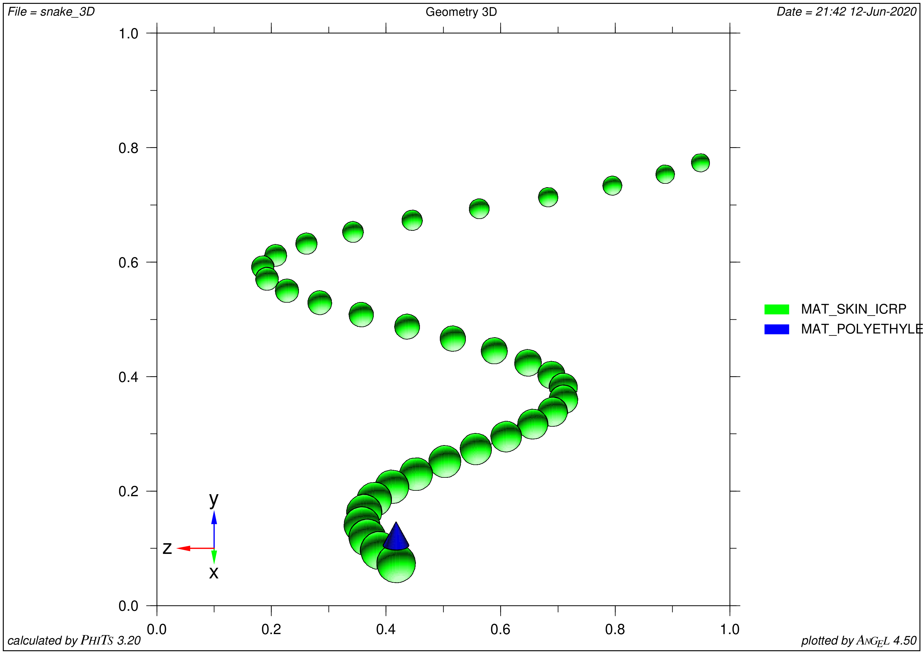
Example 2(b): Snake! PHITS visualization

Example 3: Snowman

Illustrative example of FitsGeo usage. Shows general workflow of creating complex geometry

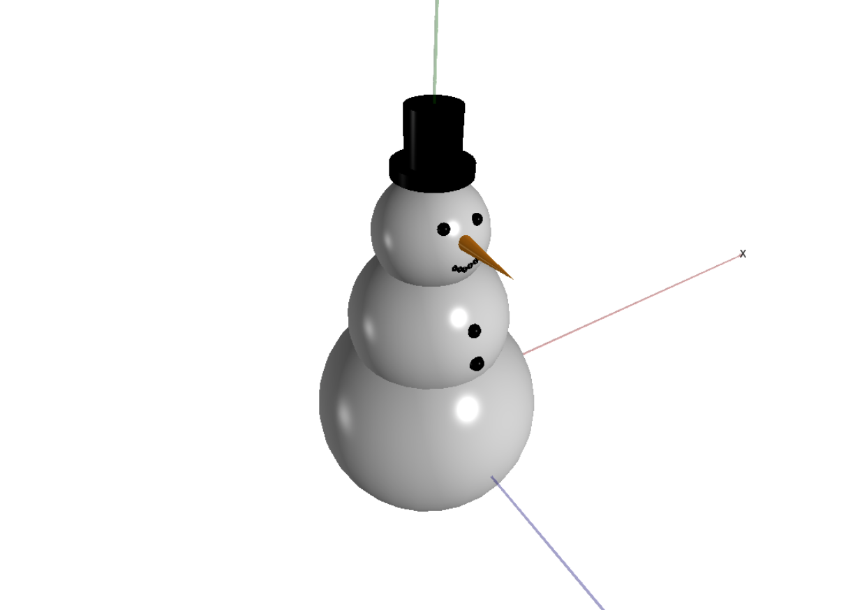
Example 3: Snowman. FitsGeo visualization

This example shows general workflow of work with FitsGeo, example contains all discussed features to build complex geometry — pretty snowman. The final result of visualization via FitsGeo is in the picture above and the full code of the example is shown below.

Example 3: Snowman

# Example 3: Snowman.
# Illustrative example of FitsGeo usage
# Shows general workflow of creating complex geometry
import fitsgeo as fg

# Create main scene, with axis
fg.create_scene(ax_length=5, background=fg.WHITE)

# Define materials
fg.MAT_WATER.color = "lightgray"
ice = fg.MAT_WATER
carbon = fg.Material.database("MAT_CARBON", color="black")
poly = fg.Material.database("MAT_PARAFFIN", color="orange")

# Create all objects for snowman
bottom = fg.SPH([0, 0, 0], 1, material=ice, name="bottom")

middle = fg.SPH(
	[bottom.x0, bottom.y0+bottom.r, bottom.z0],
	bottom.r/1.5, material=ice, name="middle")

top = fg.SPH(
	[
		middle.x0,
		middle.y0+middle.r*1.2,
		middle.z0],
	middle.r/1.5, material=ice, name="top")

carrot = fg.TRC(
	[
		top.x0,
		top.y0+top.r/4,
		top.z0+top.r/2],
	[0, 0, top.diameter*0.8], top.r/6, 1e-3, material=poly)

hat_bottom = fg.RCC(
	[top.x0, top.y0+top.r, top.z0],
	[top.x0, middle.r/7, top.z0],
	top.r/1.5, material=carbon, name="Hat bottom")

hat_top = fg.RCC(
	[
		hat_bottom.get_center[0],
		hat_bottom.get_center[1]+hat_bottom.get_len_h/2,
		hat_bottom.get_center[2]],
	[hat_bottom.get_center[0], hat_bottom.get_len_h*4, hat_bottom.get_center[2]],
	hat_bottom.r/1.5, material=carbon, name="Hat top")

eye_l = fg.SPH(
	[
		top.x0 - top.r*0.3,
		top.y0 + top.r/2,
		top.z0 + top.r*0.8],
	top.r/10, material=carbon, name="Left Eye")

eye_r = fg.SPH(
	[
		top.x0 + top.r*0.3,
		top.y0 + top.r/2,
		top.z0 + top.r*0.8],
	eye_l.r, material=carbon, name="Right Eye")

button1 = fg.SPH(
	[
		middle.x0,
		middle.y0 + middle.r*0.4,
		middle.z0 + middle.r*0.9],
	eye_r.r*1.2, material=carbon, name="Button1")

button2 = fg.SPH(
	[
		middle.x0,
		middle.y0,
		middle.z0 + middle.r],
	button1.r*1.1, material=carbon, name="Button2")

mouth1 = fg.T(
	[
		top.x0,
		top.y0*0.95,
		top.z0 + top.r],
	top.r/30, eye_l.r/7, eye_l.r/5,
	name="Mouth 1", material=carbon, rot="z")

mouth2 = fg.T(
	[
		top.x0 + 3*mouth1.r,
		top.y0*0.95 + 1.1*mouth1.r,
		top.z0 + top.r],
	mouth1.r, eye_l.r/7, eye_l.r/5,
	name="Mouth 2", material=carbon, rot="z")

mouth3 = fg.T(
	[
		top.x0 - 3*mouth1.r,
		top.y0*0.95 + 1.1*mouth1.r,
		top.z0 + top.r],
	mouth1.r, eye_l.r/7, eye_l.r/5,
	name="Mouth 3", material=carbon, rot="z")

mouth4 = fg.T(
	[
		mouth3.x0 - 3*mouth1.r,
		mouth3.y0 + 1.5*mouth1.r,
		mouth3.z0],
	mouth1.r, eye_l.r/7, eye_l.r/5,
	name="Mouth 4", material=carbon, rot="z")

mouth5 = fg.T(
	[
		mouth2.x0 + 3*mouth1.r,
		mouth2.y0 + 1.5*mouth1.r,
		mouth2.z0],
	mouth1.r, eye_l.r/7, eye_l.r/5,
	name="Mouth 5", material=carbon, rot="z")

outer = fg.SPH(r=3, name="Outer edge", material=fg.MAT_VOID)

# Create cells
outer_c = fg.Cell([+outer], "Outer Void", fg.MAT_OUTER)
inner_c = fg.Cell(
	[-outer + +bottom + +middle + +top + +hat_bottom + +hat_top + +carrot +
	 	+eye_l + +eye_r + +button1 + +button2 +
	 	+mouth1 + +mouth2 + +mouth3 + +mouth4 + +mouth5],
	"Inner Cell", fg.MAT_VOID)
bottom_c = fg.Cell([-bottom + +middle], "Bottom Cell", ice)
middle_c = fg.Cell(
	[-middle + +button1 + +button2 + +top], "Middle Cell", ice)
top_c = fg.Cell(
	[-top + +carrot + +eye_l + +eye_r],
	"Top Cell", ice)

buttons = []
for btn in [button1, button2]:
	buttons.append(fg.Cell([-btn], f"{btn.name} Cell", carbon, btn.volume))

mouth = []
for m in [mouth1, mouth2, mouth3, mouth4, mouth5]:
	mouth.append(fg.Cell([-m], f"{m.name} Cell", carbon, m.get_volume))

eyes = []
for eye in [eye_l, eye_r]:
	eyes.append(fg.Cell([-eye], f"{eye.name} Cell", carbon, eye.volume))

carrot_c = fg.Cell([-carrot], "Carrot Cell", poly, carrot.get_volume)

hat = []
for h in [hat_bottom, hat_top]:
	hat.append(fg.Cell([-h], f"{h.name} Cell", carbon, h.get_volume))

# Draw all defined objects
for s in [s for s in fg.created_surfaces if s is not carrot]:
	s.draw()

carrot.draw(truncated=False)

# Export all drawn surfaces to PHITS input sections
fg.phits_export(to_file=True, inp_name="snowman")

The main idea in this example was to make the bottom snowball of snowman and to set every other part of snowman relative to this object. This example doesn’t need any additional commentaries, every feature was discussed in the previous examples. Just try to run the example and look carefully how the geometry was set in the code.

Full PHITS input file and visualization of geometry via ANGEL are shown below. The highlighted part of the code — exported sections from FitsGeo.

Example 3: Snowman. PHITS input

[ Title ]
	Snowman (Example3): one more example of how to use FitsGeo module
	Illustrative example of FitsGeo usage
	Shows general workflow

[ Parameters ]
	icntl = 11			# (D=0) 3:ECH 5:ALL VOID 6:SRC 7,8:GSH 11:DSH 12:DUMP

[ Source ]
	s-type = 2			# mono-energetic rectangular source 
	e0 = 1				# energy of beam [MeV]
	proj = proton		# kind of incident particle

[ Material ]
    mat[1] H 2.0 O 1.0  GAS=0 $ name: 'MAT_WATER'
    mat[2] C 6.0  GAS=0 $ name: 'MAT_CARBON'
    mat[3] H 2.0 C 1.0  GAS=0 $ name: 'MAT_PARAFFIN'

[ Mat Name Color ]
    mat name    size    color
    1   {MAT\_WATER}    1.00    lightgray
    2   {MAT\_CARBON}   1.00    black
    3   {MAT\_PARAFFIN} 1.00    orange

[ Surface ]
    1   SPH  0 0 0  1 $ name: 'bottom' (sphere) x0 y0 z0 R
    2   SPH  0 1 0  0.6666666666666666 $ name: 'middle' (sphere) x0 y0 z0 R
    3   SPH  0 1.7999999999999998 0  0.4444444444444444 $ name: 'top' (sphere) x0 y0 z0 R
    4   TRC  0 1.911111111111111 0.2222222222222222  0 0 0.7111111111111111  0.07407407407407407  0.001 $ name: 'RCC' (truncated right-angle cone) [x0 y0 z0] [Hx Hy Hz] R_b R_t
    5   RCC  0 2.2444444444444445 0  0 0.09523809523809523 0  0.2962962962962963 $ name: 'Hat bottom' (cylinder) [x0 y0 z0] [Hx Hy Hz] R
    6   RCC  0.0 2.3396825396825394 0.0  0.0 0.38095238095238093 0.0  0.19753086419753085 $ name: 'Hat top' (cylinder) [x0 y0 z0] [Hx Hy Hz] R
    7   SPH  -0.13333333333333333 2.022222222222222 0.35555555555555557  0.04444444444444444 $ name: 'Left Eye' (sphere) x0 y0 z0 R
    8   SPH  0.13333333333333333 2.022222222222222 0.35555555555555557  0.04444444444444444 $ name: 'Right Eye' (sphere) x0 y0 z0 R
    9   SPH  0 1.2666666666666666 0.6  0.05333333333333332 $ name: 'Button1' (sphere) x0 y0 z0 R
    10   SPH  0 1 0.6666666666666666  0.05866666666666666 $ name: 'Button2' (sphere) x0 y0 z0 R
    11   TZ  0 1.7099999999999997 0.4444444444444444  0.014814814814814814  0.006349206349206348  0.008888888888888887 $ name: 'Mouth 1' (torus, with z rotational axis) [x0 y0 z0] A(R) B C
    12   TZ  0.04444444444444444 1.726296296296296 0.4444444444444444  0.014814814814814814  0.006349206349206348  0.008888888888888887 $ name: 'Mouth 2' (torus, with z rotational axis) [x0 y0 z0] A(R) B C
    13   TZ  -0.04444444444444444 1.726296296296296 0.4444444444444444  0.014814814814814814  0.006349206349206348  0.008888888888888887 $ name: 'Mouth 3' (torus, with z rotational axis) [x0 y0 z0] A(R) B C
    14   TZ  -0.08888888888888888 1.7485185185185181 0.4444444444444444  0.014814814814814814  0.006349206349206348  0.008888888888888887 $ name: 'Mouth 4' (torus, with z rotational axis) [x0 y0 z0] A(R) B C
    15   TZ  0.08888888888888888 1.7485185185185181 0.4444444444444444  0.014814814814814814  0.006349206349206348  0.008888888888888887 $ name: 'Mouth 5' (torus, with z rotational axis) [x0 y0 z0] A(R) B C
    16   SPH  0.0 0.0 0.0  3 $ name: 'Outer edge' (sphere) x0 y0 z0 R

[ Cell ]
    100 -1  (16) $ name: 'Outer Void' 

    101 0  (-16 1 2 3 5 6 4 7 8 9 10 11 12 13 14 15) $ name: 'Inner Cell' 

    102 1  1.0  (-1 2)   $ name: 'Bottom Cell' 
    103 1  1.0  (-2 9 10 3)   $ name: 'Middle Cell' 
    104 1  1.0  (-3 4 7 8)   $ name: 'Top Cell' 
    105 2  2.0  (-9)  VOL=0.0006354549881038906 $ name: 'Button1 Cell' 
    106 2  2.0  (-10)  VOL=0.0008457905891662785 $ name: 'Button2 Cell' 
    107 2  2.0  (-11)  VOL=1.6504139569396266e-05 $ name: 'Mouth 1 Cell' 
    108 2  2.0  (-12)  VOL=1.6504139569396266e-05 $ name: 'Mouth 2 Cell' 
    109 2  2.0  (-13)  VOL=1.6504139569396266e-05 $ name: 'Mouth 3 Cell' 
    110 2  2.0  (-14)  VOL=1.6504139569396266e-05 $ name: 'Mouth 4 Cell' 
    111 2  2.0  (-15)  VOL=1.6504139569396266e-05 $ name: 'Mouth 5 Cell' 
    112 2  2.0  (-7)  VOL=0.00036774015515271454 $ name: 'Left Eye Cell' 
    113 2  2.0  (-8)  VOL=0.00036774015515271454 $ name: 'Right Eye Cell' 
    114 3  0.89  (-4)  VOL=0.004141907421006144 $ name: 'Carrot Cell' 
    115 2  2.0  (-5)  VOL=0.026267153939479614 $ name: 'Hat bottom Cell' 
    116 2  2.0  (-6)  VOL=0.04669716255907488 $ name: 'Hat top Cell' 

[ T-3Dshow ]
	title = Geometry 3D
	x0 = 0
	y0 = 1
	z0 = 0

	w-wdt = 4
	w-hgt = 4
	w-dst = 10

	w-mnw = 400		# Number of meshes in horizontal direction.
	w-mnh = 400		# Number of meshes in vertical direction.
	w-ang = 0

	e-the = 40
	e-phi = 120
	e-dst = 100

	l-the = 80
	l-phi = 140
	l-dst = 200*100

	file = snowman_3D
	output = 3		# (D=3) Region boundary + color
	width = 0.5		# (D=0.5) The option defines the line thickness.

	epsout = 1

[ E n d ]

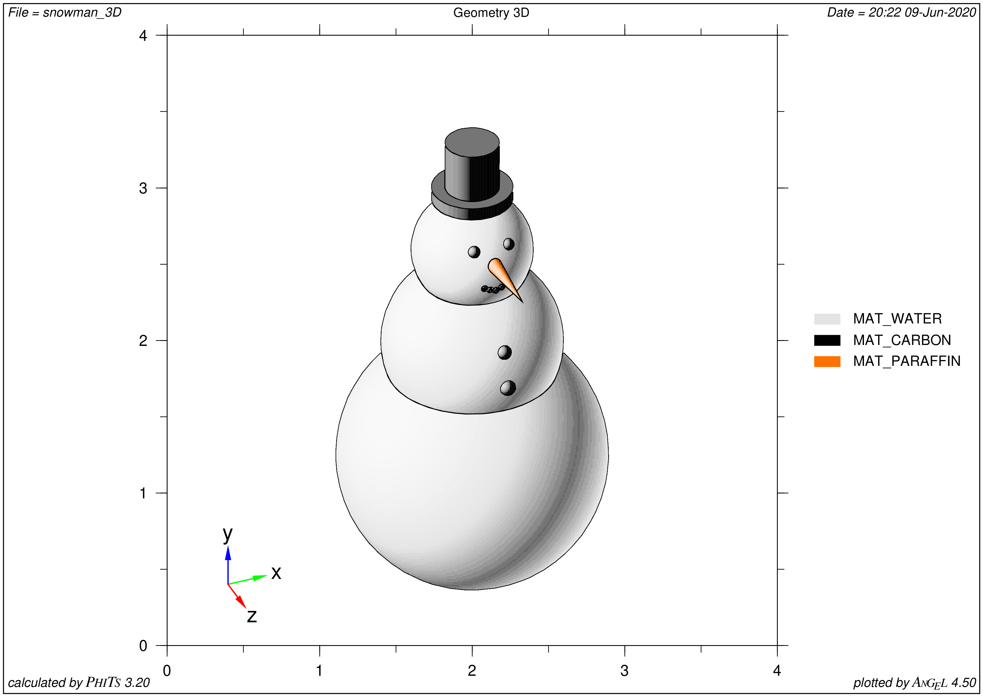
Example 3: Snowman. PHITS visualization